Fun with Frequencies
CS 194-26 Project #3 · Owen Jow · September 2016
Part 0: Image Sharpening
Here, we will sharpen a few images by making use of the unsharp mask filter. At a high level, this means creating an edge representation of an image and adding a scaled version of it to the original. The idea is that blurring takes away detail (i.e. what we think of as edges, mostly) from an image – so to sharpen, all we have to do is add that detail back. Mathematically, we have the following relationship:
original + α(detail) = sharpened
where α is a scaling factor.
How do we get the edge representation? That's where unsharp masking comes in. We'll first obtain a low-passed ("unsharp") version of the image by convolving it with a 2D Gaussian filter. Then, to retain only the components in the image with higher frequencies, we'll subtract our unsharp version of the image from the original. Finally, once we have the high-frequency image, we can scale it and add it to the OG image in order to arrive at our sharpened result.
If
f is the input image,
g is our 2D Gaussian kernel, and
e is the unit impulse, then
sharpened = f + α(f - f * g) = f * ((1 + α)e - αg)
Note that
* is the convolution operator. Also note that we have some choice in how we construct the Gaussian filter; we're able to select both the kernel width and the standard deviation (σ) of the curve. In all of the following cases, I use a 20x20 kernel and a σ of 5, as these values seemed to give the best results.
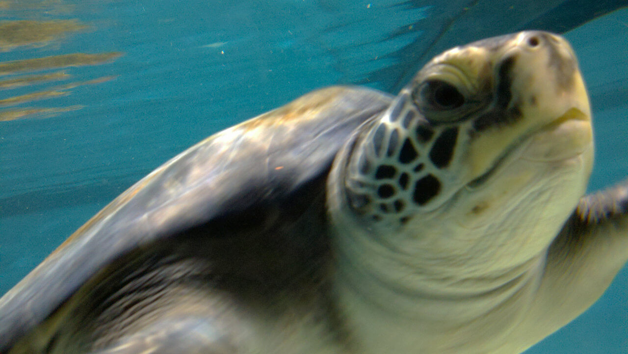
Turtle (before)
|
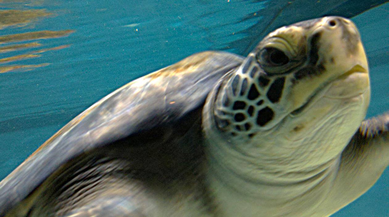
Turtle (after)
|
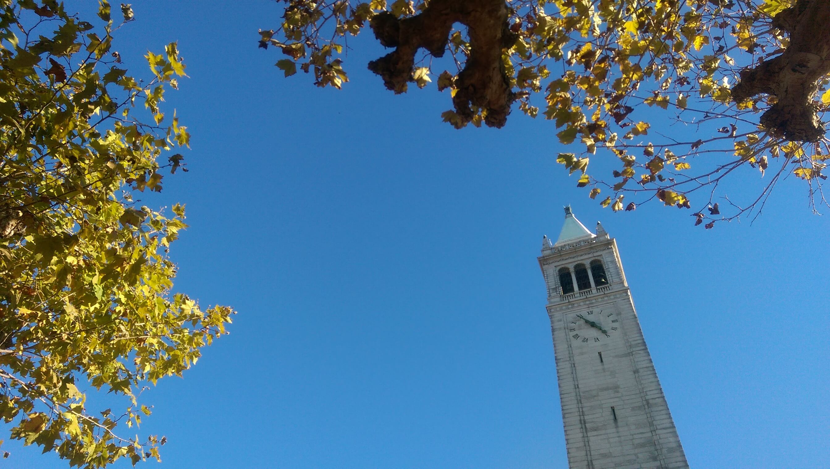
Campanile (before)
|
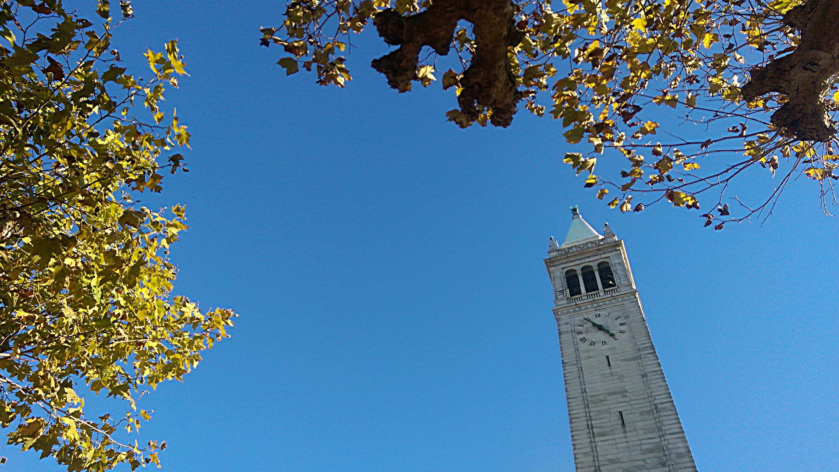
Campanile (after)
|
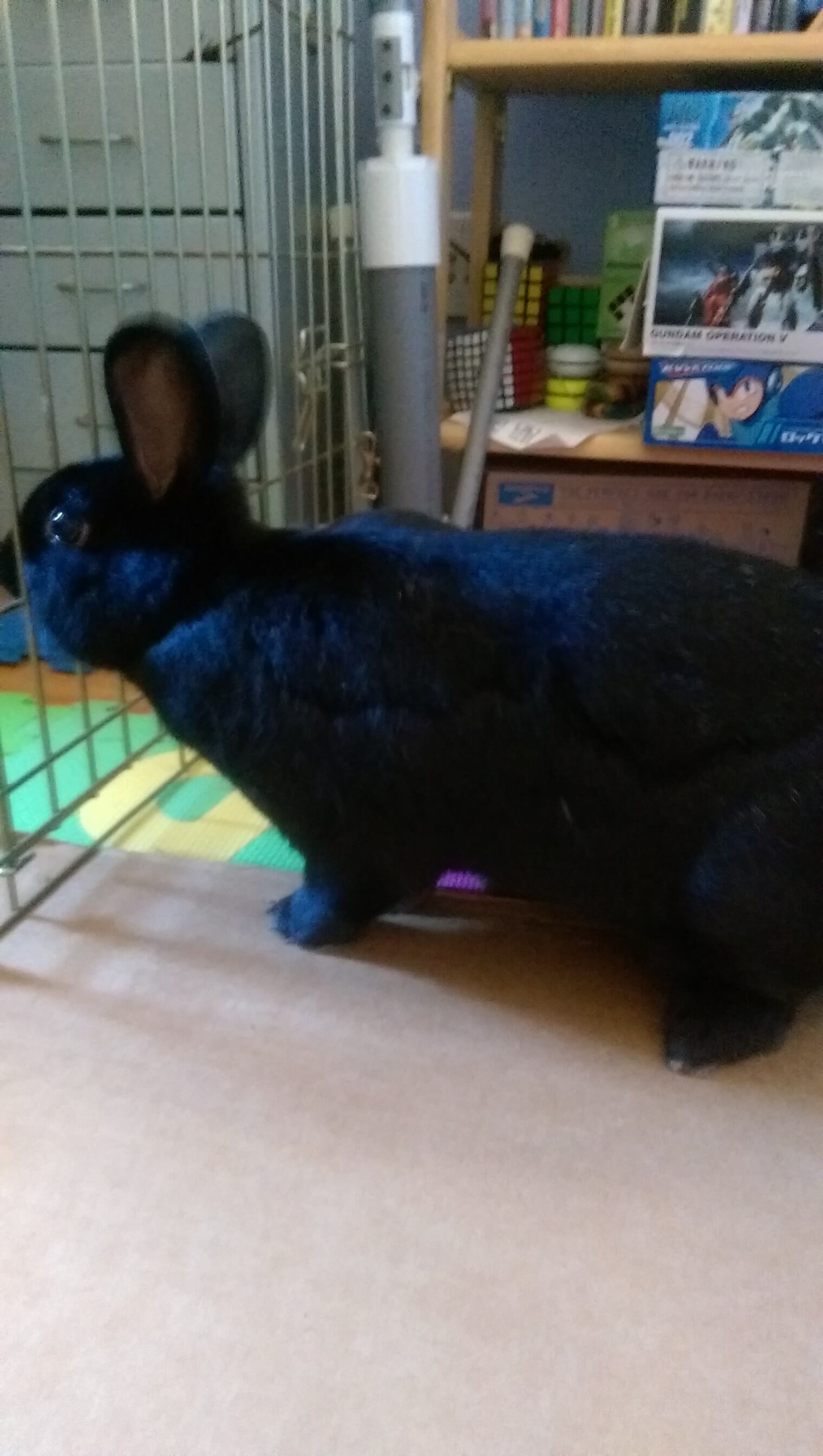
Dennis (before)
|

Dennis (after)
|
Part 1: Hybrid Images
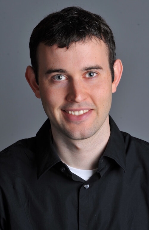
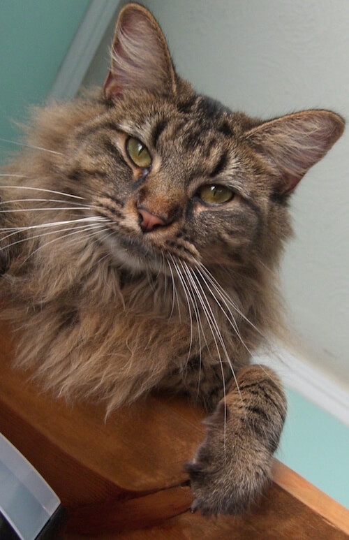
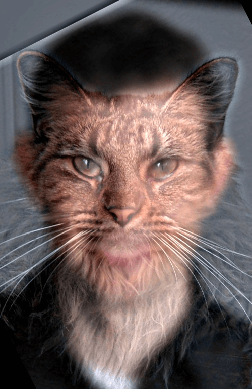
A hybrid image is defined as a static image that changes in interpretation as a function of the viewing distance. It is created by combining the low-frequency version of one image with the high-frequency version of another. From up close, the high frequencies dominate the image, but when viewed from afar, the low frequencies take over because they're the only thing a person can see. Below is an example of Derek hybridized with his cat Nutmeg. In it, we retain the low-passed version of Derek and the high-passed version of Nutmeg.
Put another way, we apply a 25x25 Gaussian filter to one image to keep only the low frequencies, and a Laplacian filter to the other to keep only the high frequencies. Added together, we have our hybrid image.
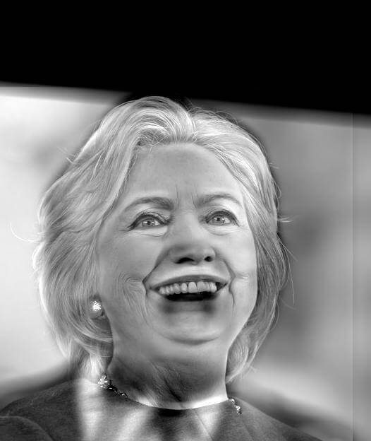
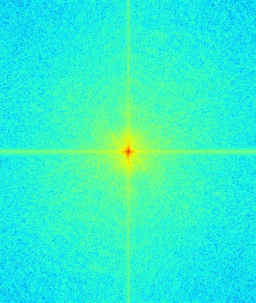
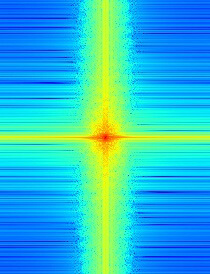
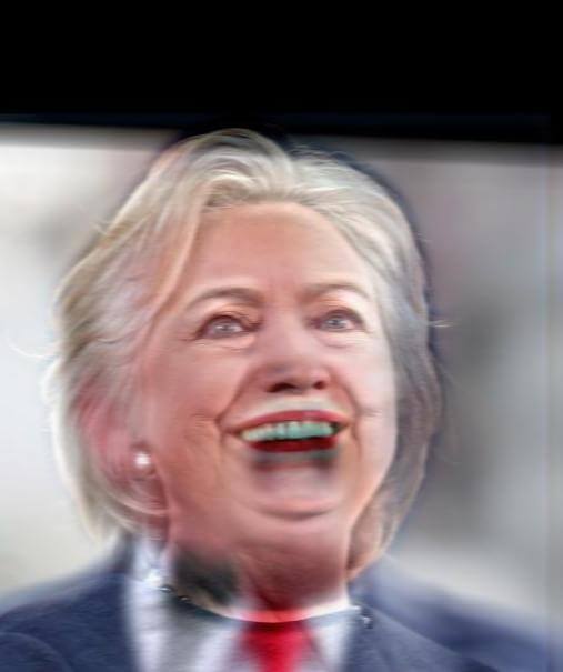
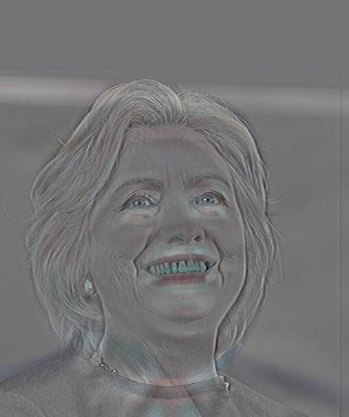
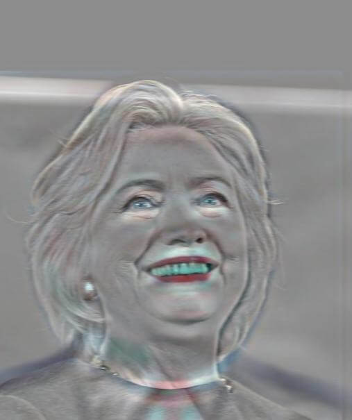
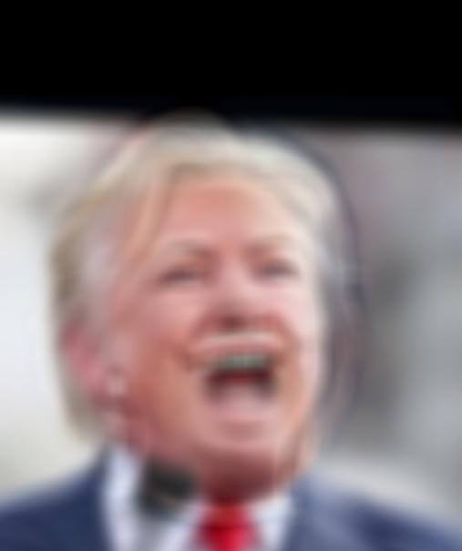
Here, we will create a hybrid of Trump and Clinton. Trump will be used as the low-frequency image, which means that Clinton will be used as his high-frequency counterpart. To the right of the images are the log magnitudes of the images' Fourier transforms, so that we can observe what happens in the frequency domain as we go. The low frequency cutoff for Trump is 0.02 Hz, while the high frequency cutoff for Clinton is 0.03 Hz.
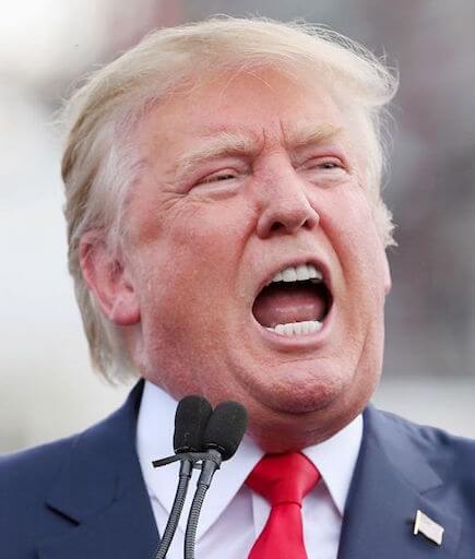
Trump (spatial domain)
|
Trump (frequency domain)
|
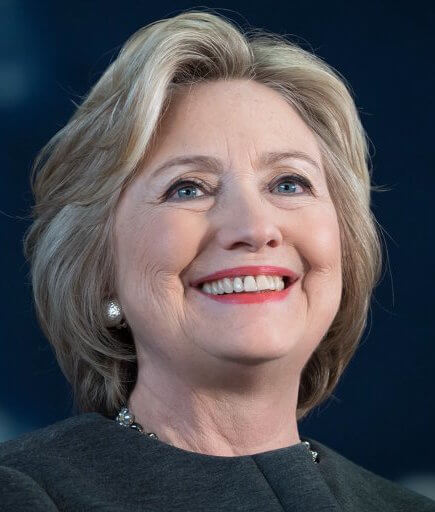
Clinton (spatial domain)
|
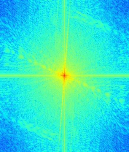
Clinton (frequency domain)
|

Low-pass (spatial domain)
|
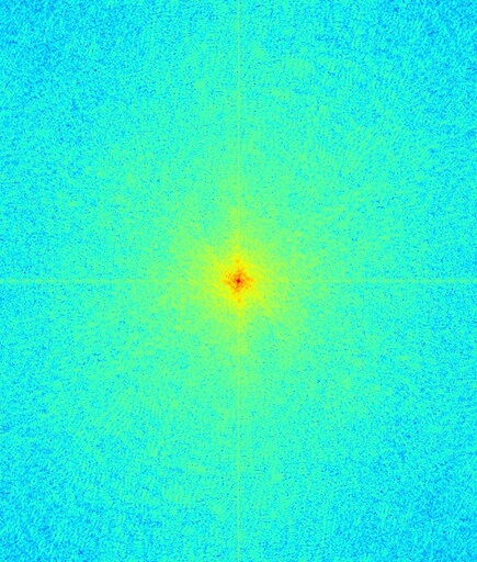
Low-pass (frequency domain)
|
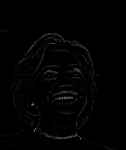
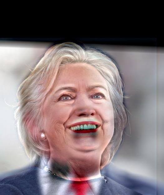
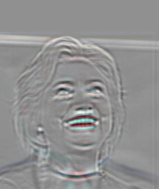
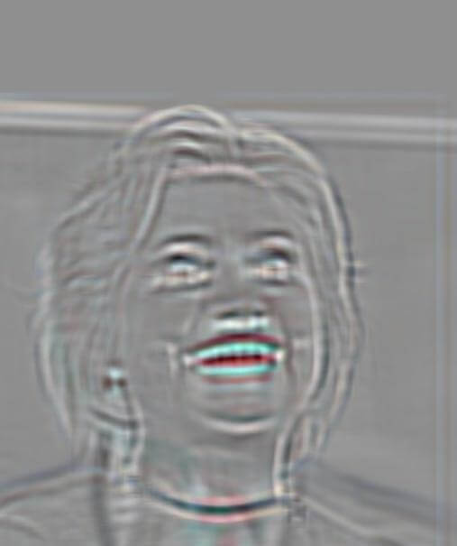
High-pass (spatial domain)
|
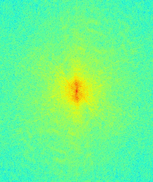
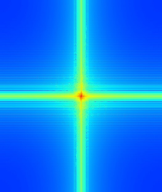
High-pass (frequency domain)
|
At this point, it is evident from the Fourier transform images that most of the high-frequency components of Trump's image have been removed. Likewise, most of the low-frequency components of Clinton's image are now gone, leaving only a frightening-looking edge image.
Hybrid image (gray)
|
FT of hybrid image
|
Hybrid image (color)
|
And at last we arrive at our hybrid image (both in grayscale and color). It's not perfect; Clinton's high-frequency image seems to overwhelm Trump's low frequencies a bit, even at a distance (specifically the eyes, which are much wider and clearer than Trump's in these pictures). In theory, it should be possible to alleviate this by selecting better frequency cutoffs and maybe retaining a different range of Clinton's features.
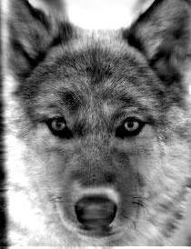
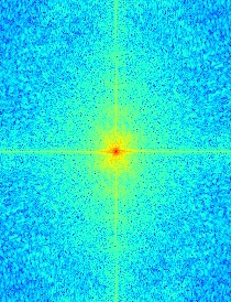
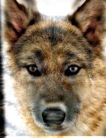
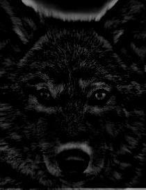
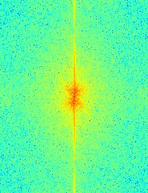
Below we have another example, which merges a dog and a wolf. This time, the low- and high-frequency cutoffs are both 0.05 Hz. The Gaussian filter is still 25x25.
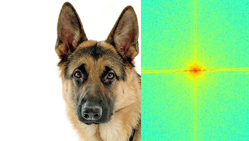
Dog + Fourier transform
|
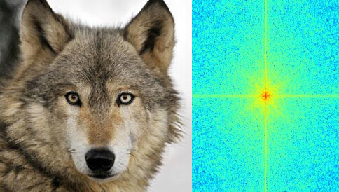
Wolf + Fourier transform
|
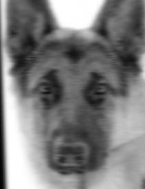
Low-pass (spatial domain)
|
Low-pass (frequency domain)
|
High-pass (spatial domain)
|
High-pass (frequency domain)
|
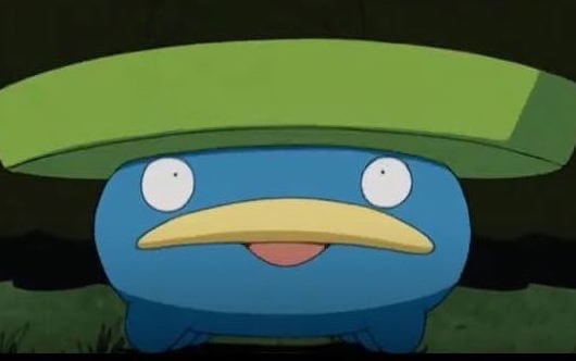
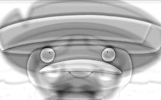
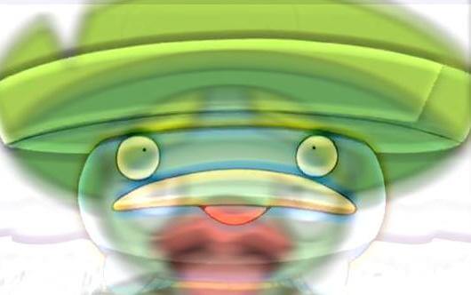
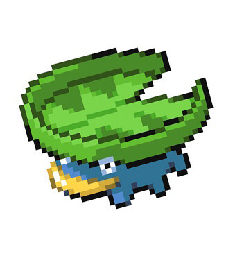
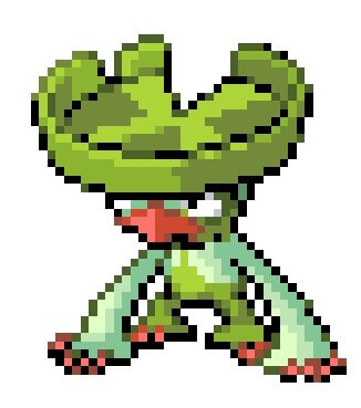
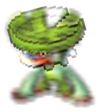
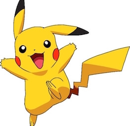
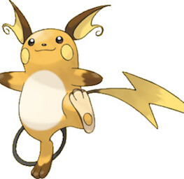
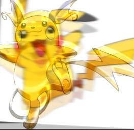
Next are a few other results of varying quality. In both of the Lotad/Lombre fusion images, the high-frequency Lotad seems to dominate a little more than would be ideal.
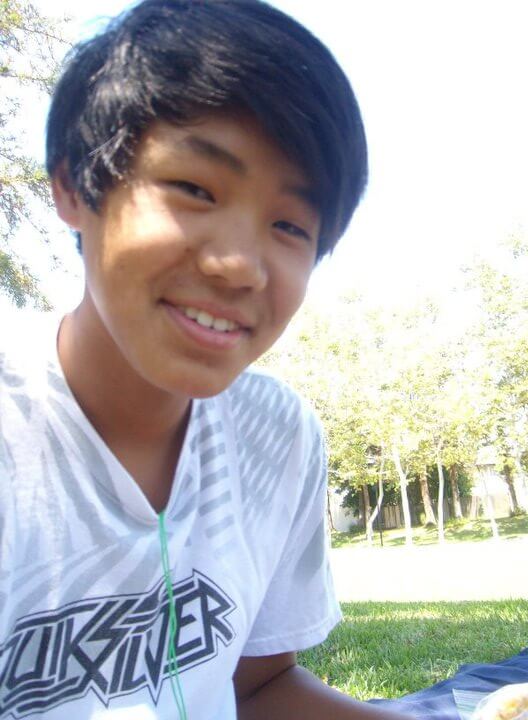
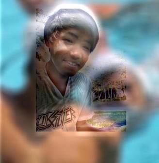
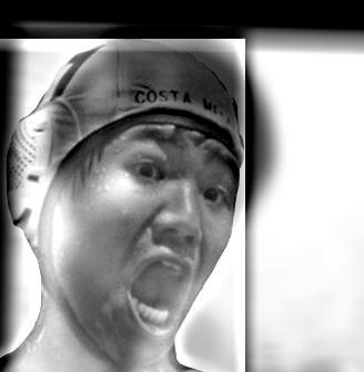
And as an example of a hybrid image that didn't work at all, we will consider the attempt to combine these two images of my roommate Sagang. Unfortunately, they ended up being too dissonant in content, and in every case it was especially difficult to distinguish the low frequencies underneath all of the high-frequency components.
Bells and Whistles
As has probably been noted, the hybrid images have also been implemented in color. This basically came down to applying the hybrid generation process on each of the color channels separately, and then stacking them together at the end. I decided to colorize both the low and high frequencies, although since color is hardly apparent in the high-passed images I don't think the high frequency colors contribute as much to the final image.
Part 2: Gaussian and Laplacian Stacks
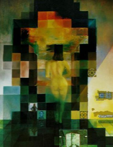
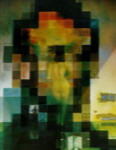
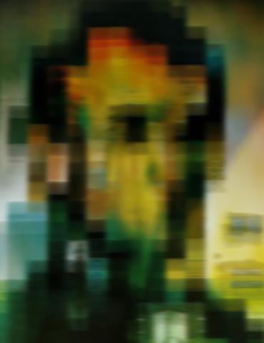
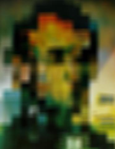
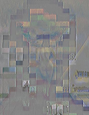
A Gaussian stack is simply the original image convolved with a bunch of Gaussian filters of increasing σ. Meanwhile, the Laplacian stack is the difference between successive levels of the Gaussian stack. Both of these, applied to Salvador Dalí's Lincoln in Dalivision lithograph, are shown below.
(All Laplacian stacks displayed in this writeup have had their images' pixel intensities normalized for easier viewing, such that the minimum value is always 0 and the maximum value is always 1.)
|
|
|
|

|
Gaussian stack (σ = 1, 2, 4, 8, 16)
|
|
|
|

|
Laplacian stack, normalized
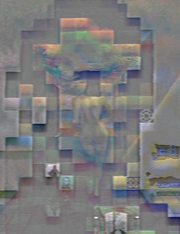
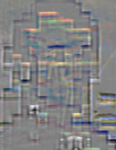
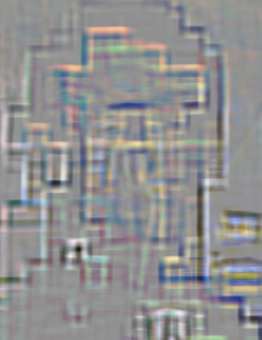
We also construct the Gaussian and Laplacian stacks for the hybrid image of Clinton and Trump. After successive blurring (i.e. the Gaussian stack), we end up getting only the lower-frequency components of Trump (which simulates what we see when we stand really far away). For the Laplacian stack, meanwhile, note that the earlier images involve higher frequencies than the later images. This allows us to isolate an edge image that's almost all Clinton.

|
|

|

|

|
Gaussian stack (σ = 1, 2, 4, 8, 16)
|
|
|
|
|
Laplacian stack, normalized
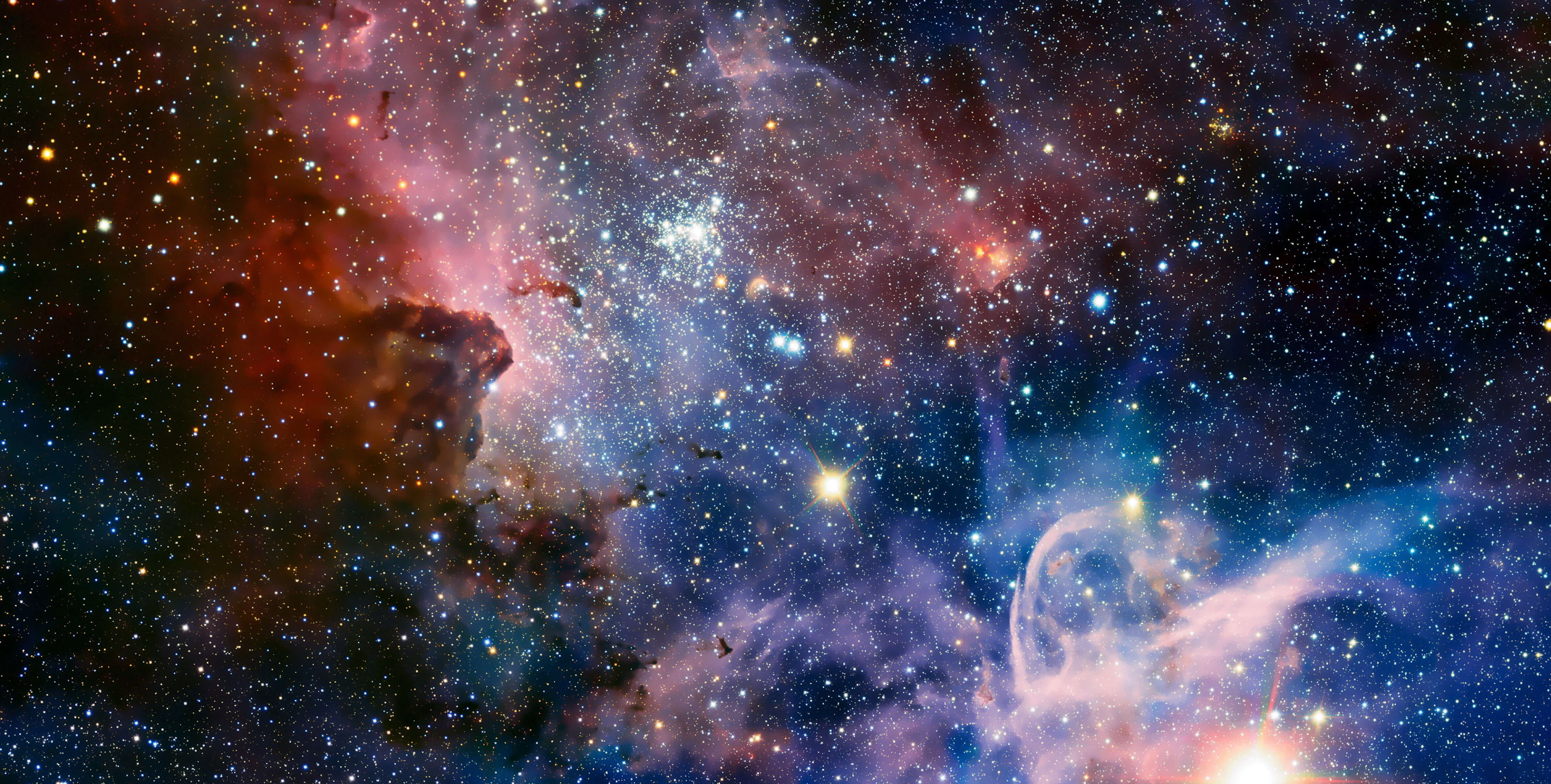
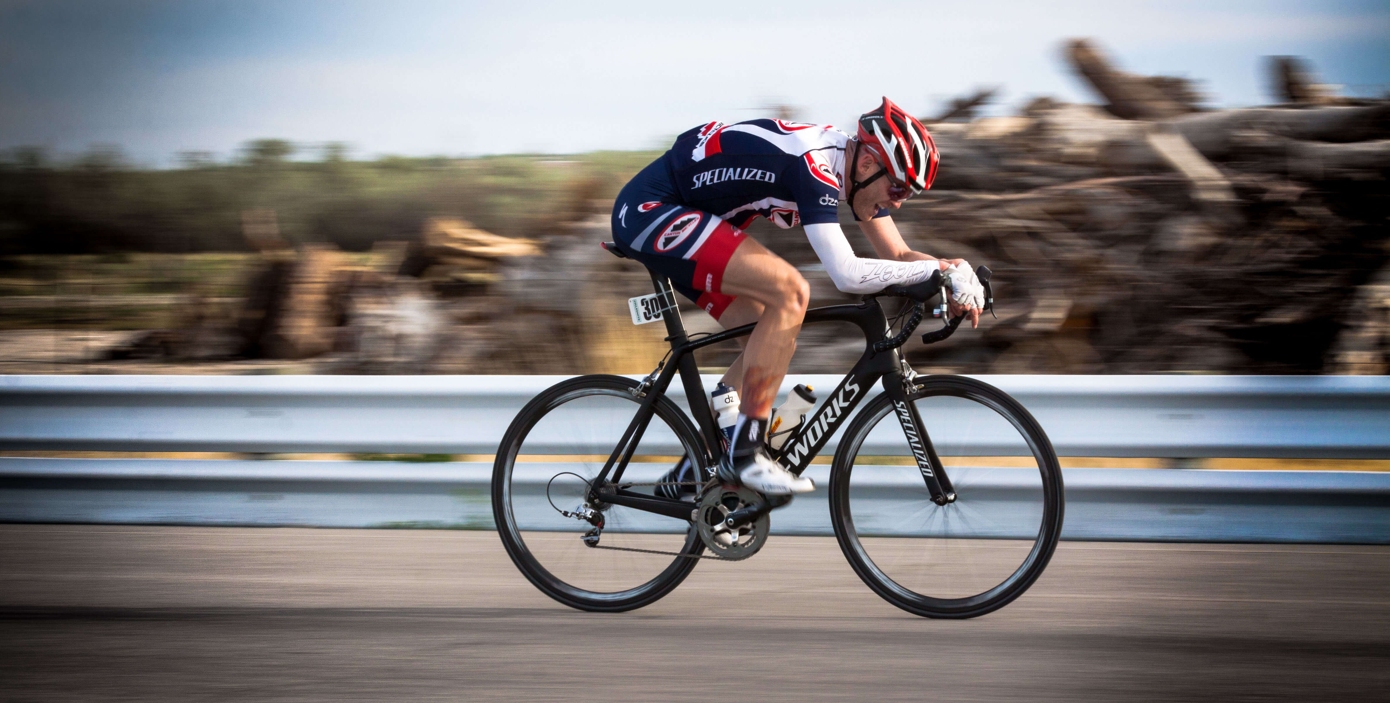
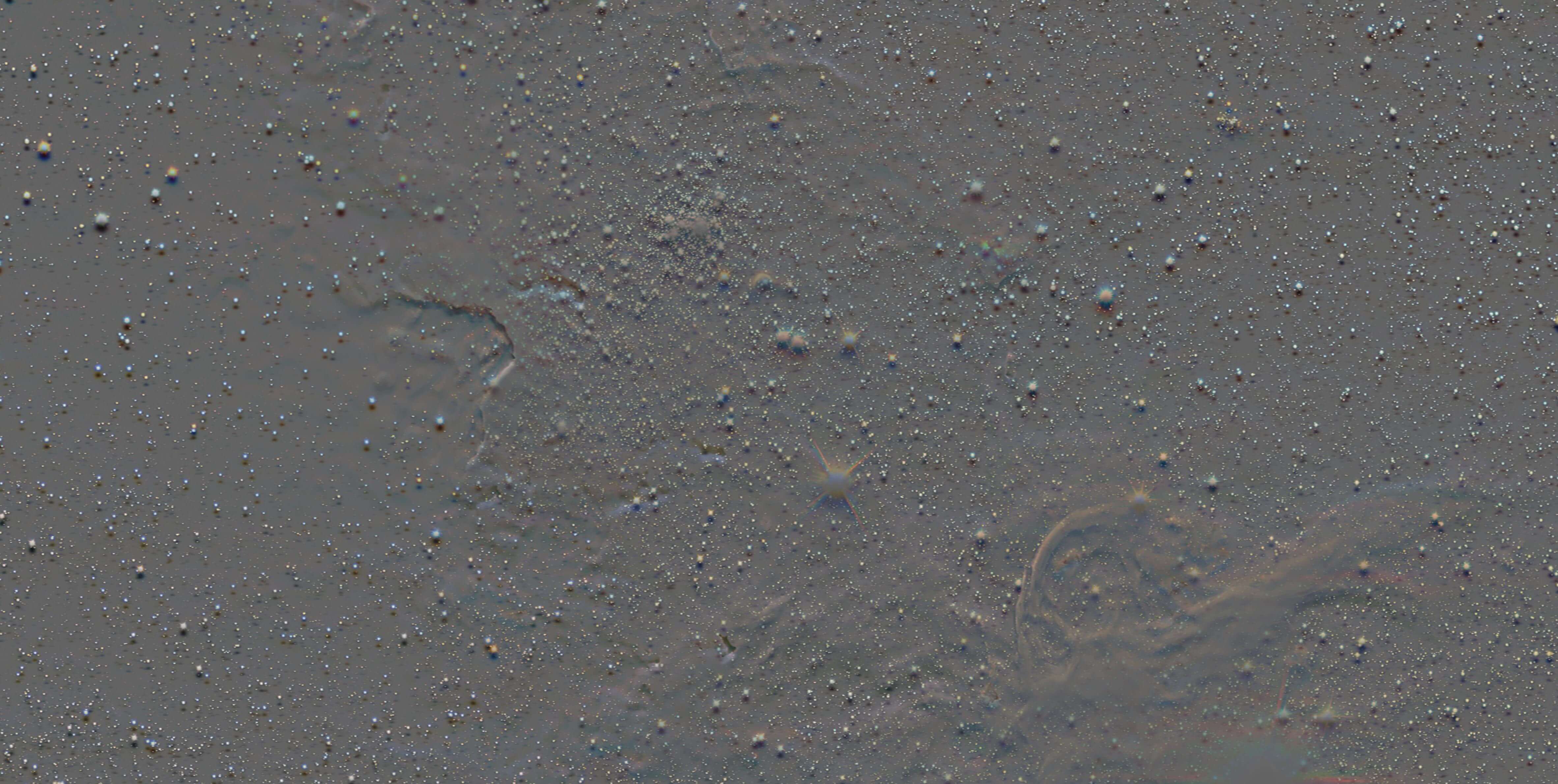
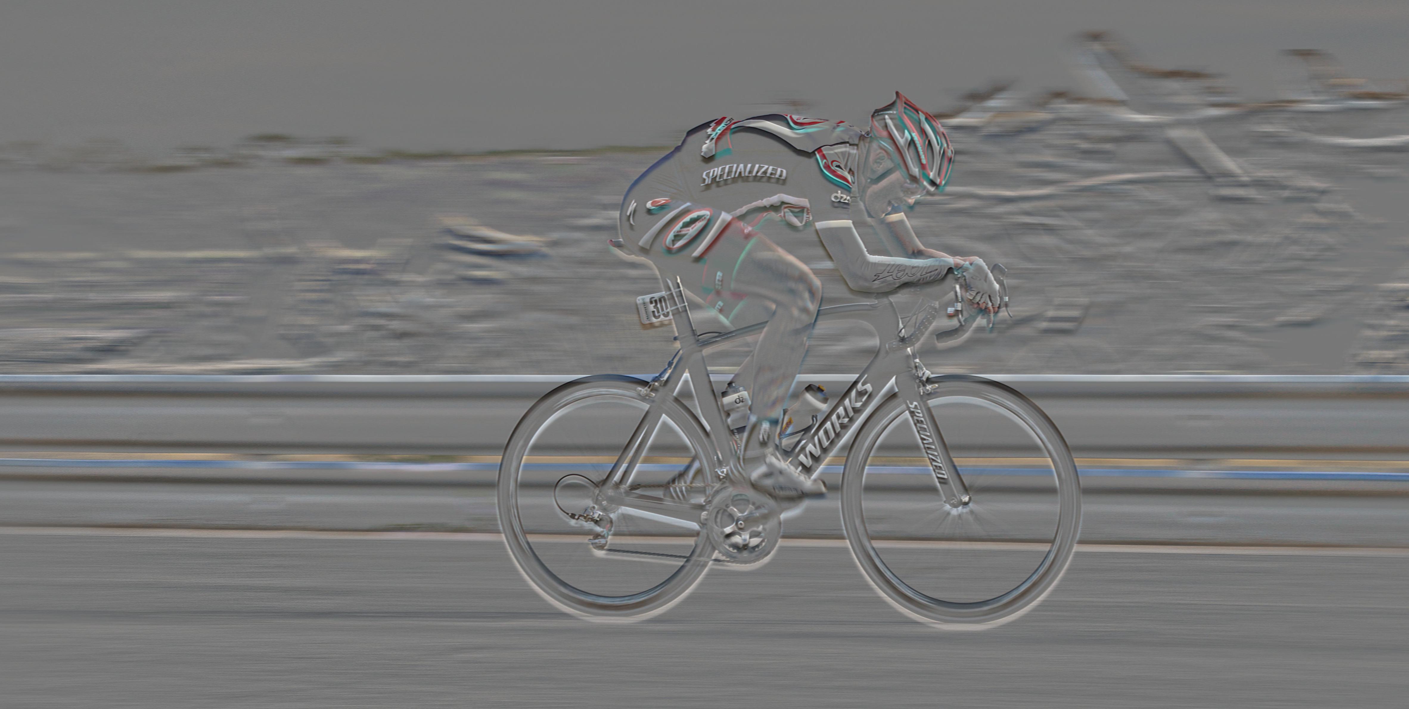
Part 3: Multiresolution Blending
As the final part of the project, we blend together two images by constructing a Laplacian stack for each of the images to be blended, and a Gaussian stack for a mask. Then each of the layers in the two Laplacian stacks are linearly combined using the corresponding layer in the Gaussian mask stack, and results from every layer are collapsed (summed together) in order to arrive at the final, blended image. This has the effect of creating a very gentle seam between each of the two images.
Parameter-wise, I used a Gaussian kernel size of 25x25, a σ of 1, and ten levels in each of the Gaussian and Laplacian stacks.
In order to obtain the following results: we take our two images, resize and align them so that they are the same resolution, and create a mask for one of them in Photoshop. The Laplacian stack for the two images and the Gaussian stack for the mask are generated... and finally we form the overall multiresolution blend by going through the process described earlier (combining stack levels and collapsing).
|
|
|
|

|
|
|

|
|
|

|
|
|

|
|
|

|
|
|

|
|
|

|
|
|
|
|

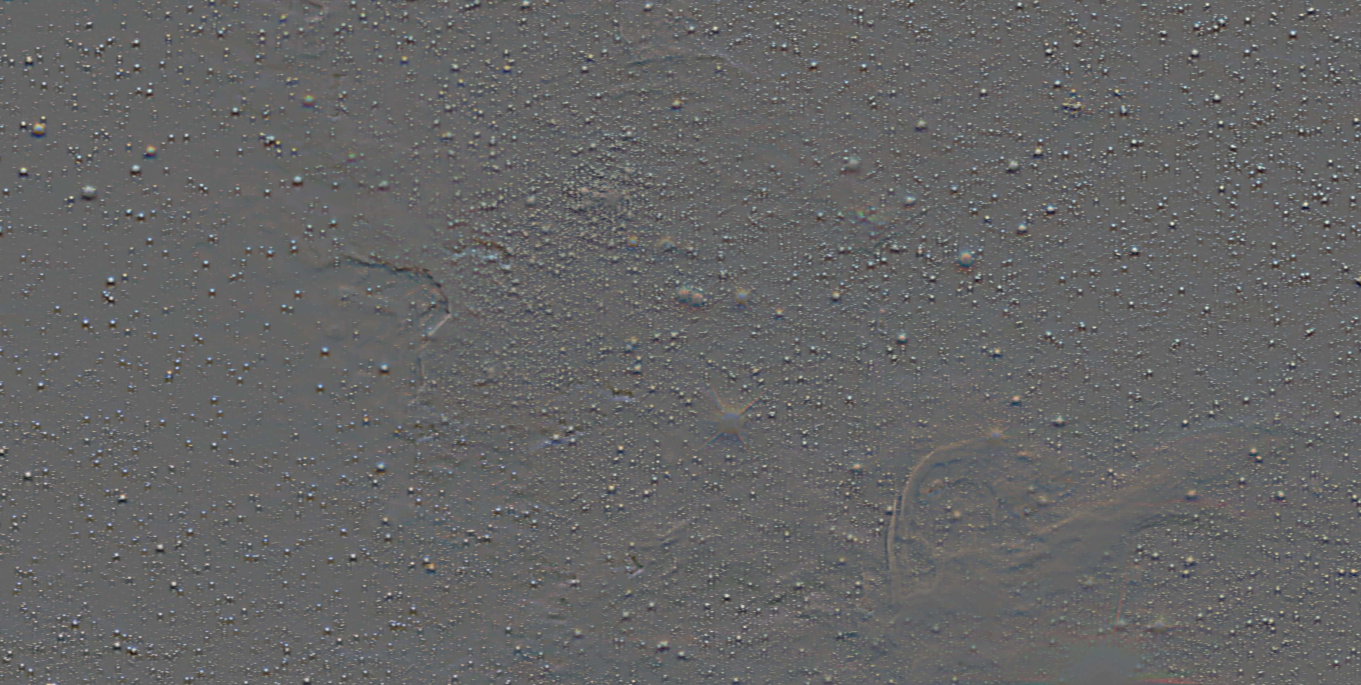
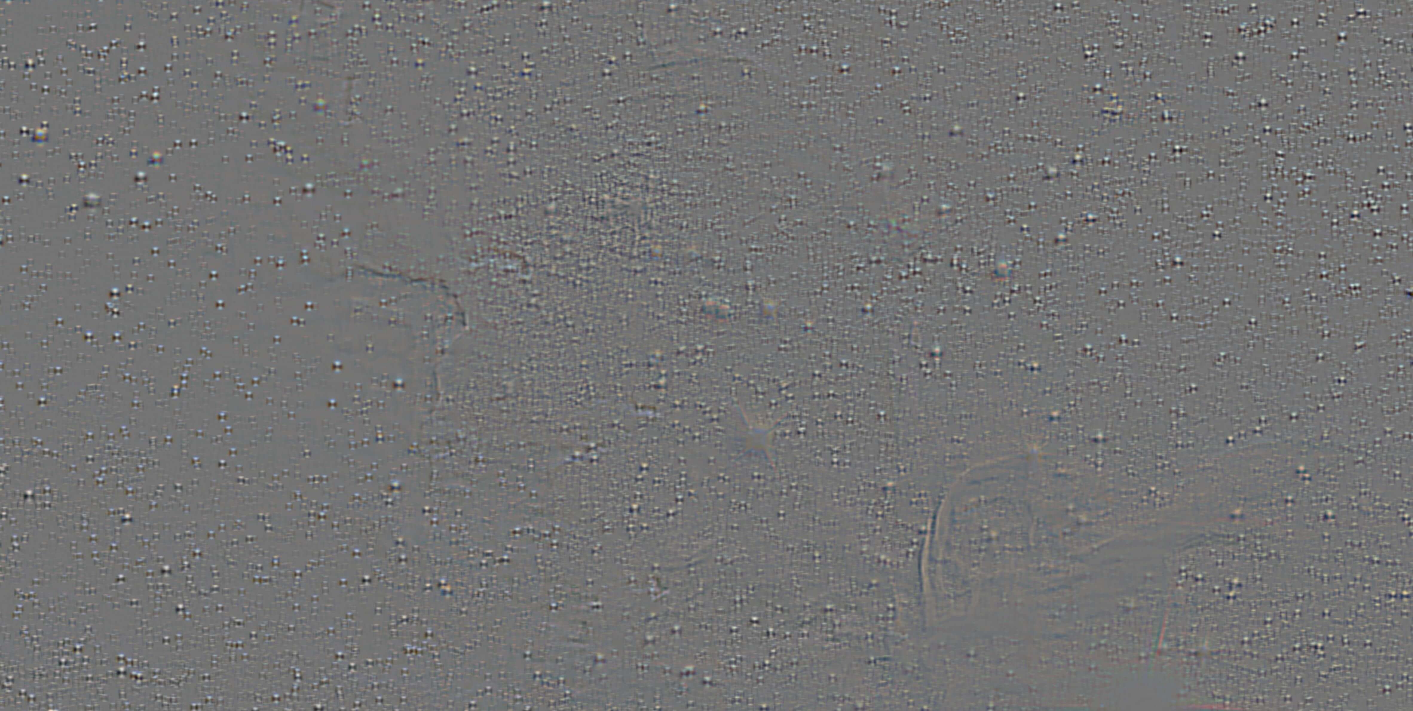
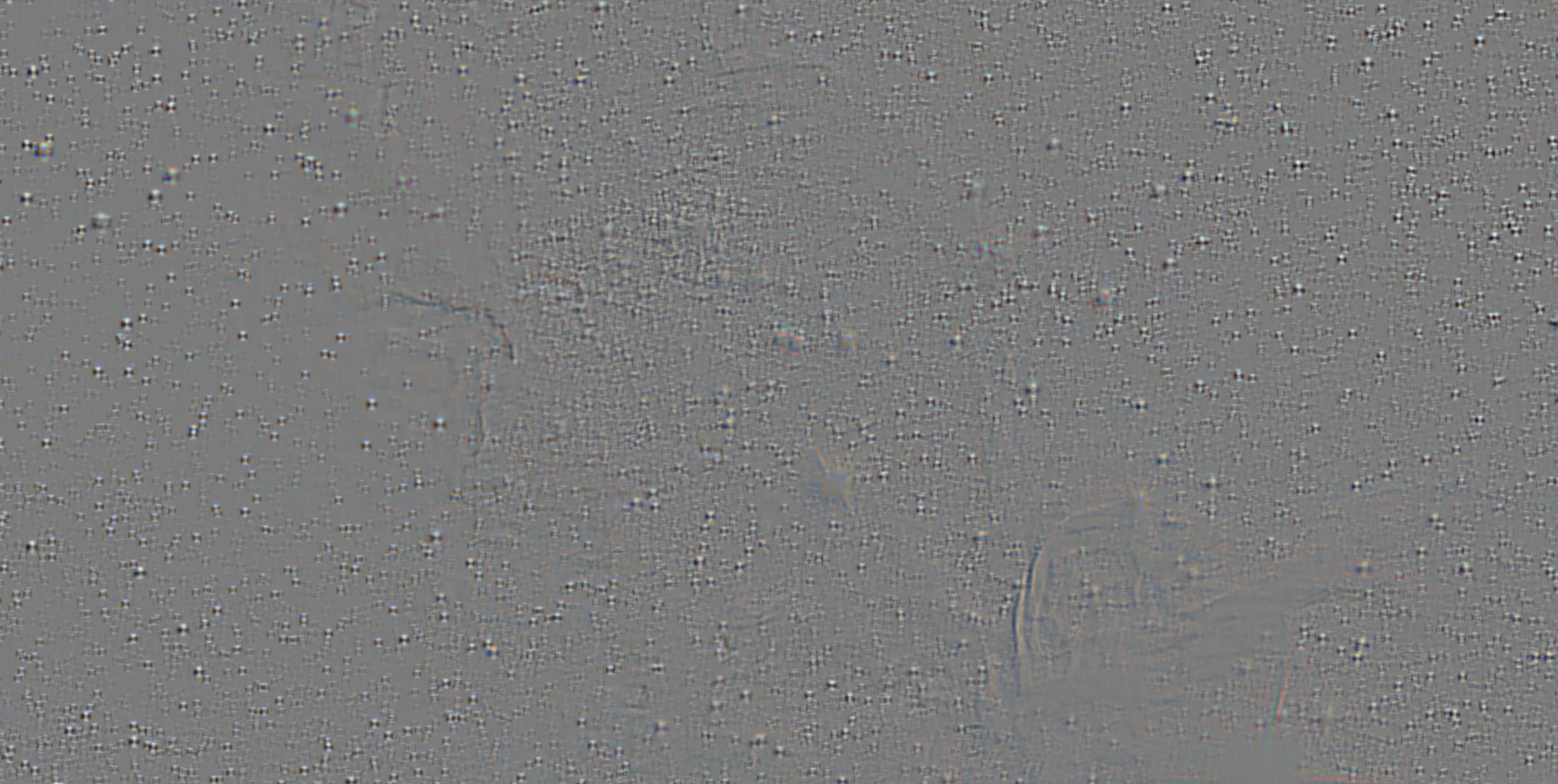
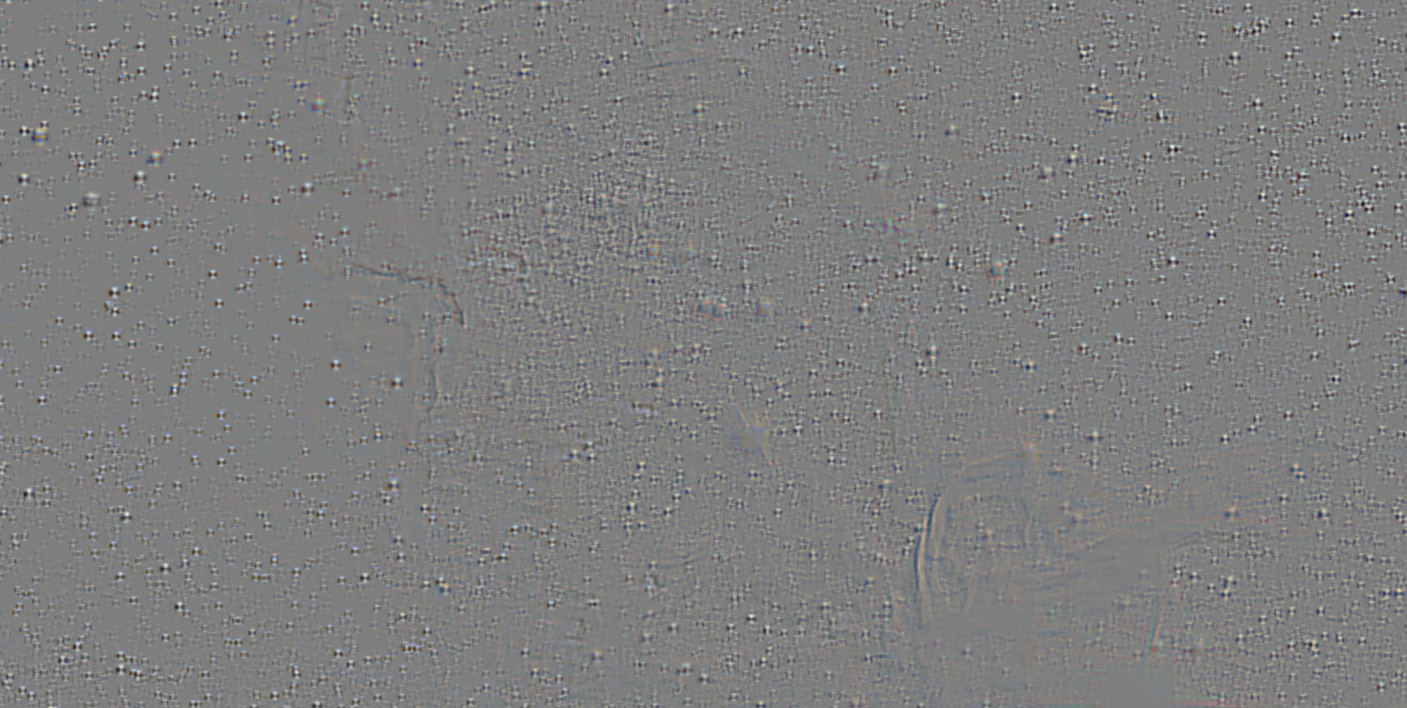
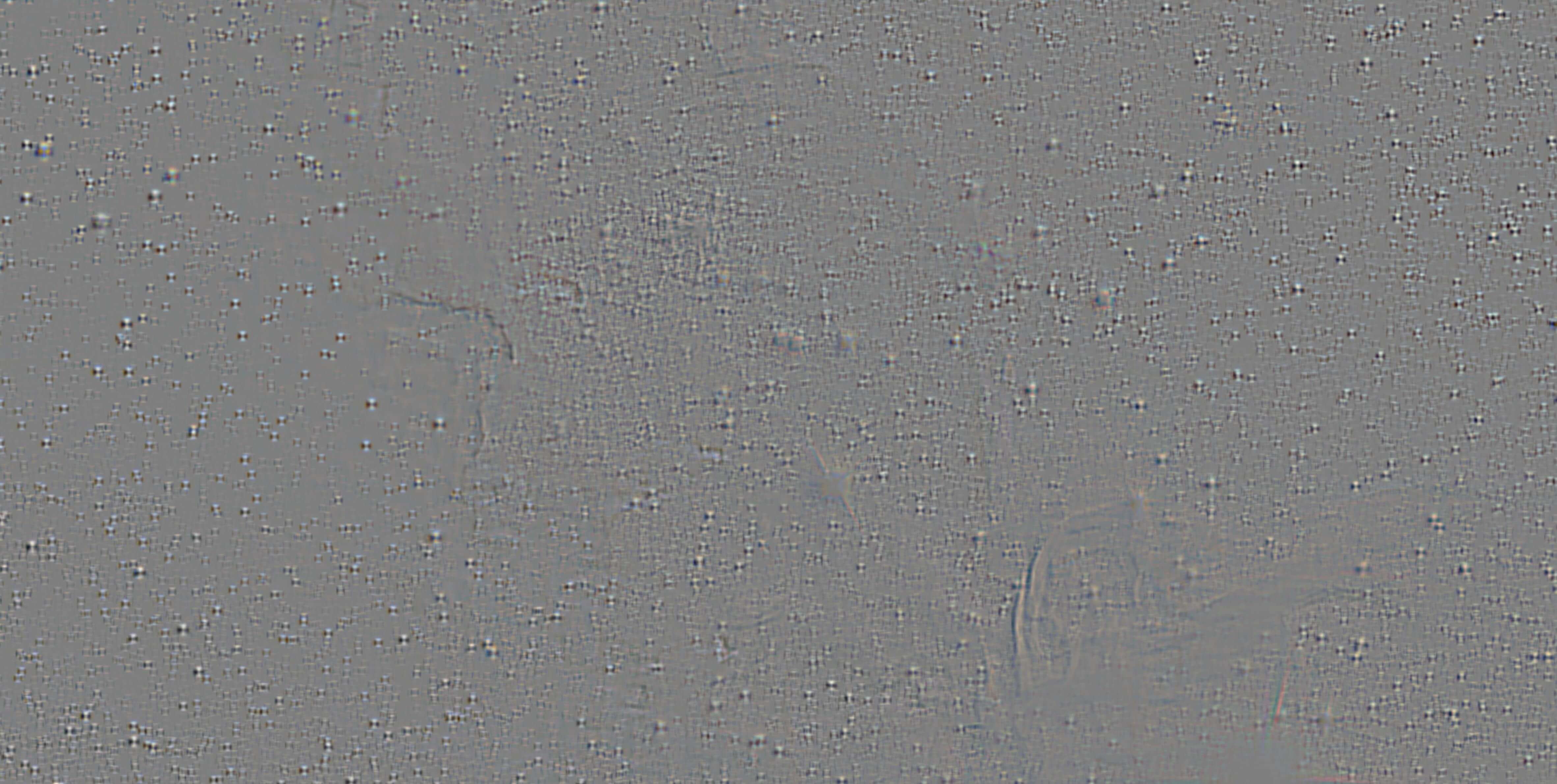
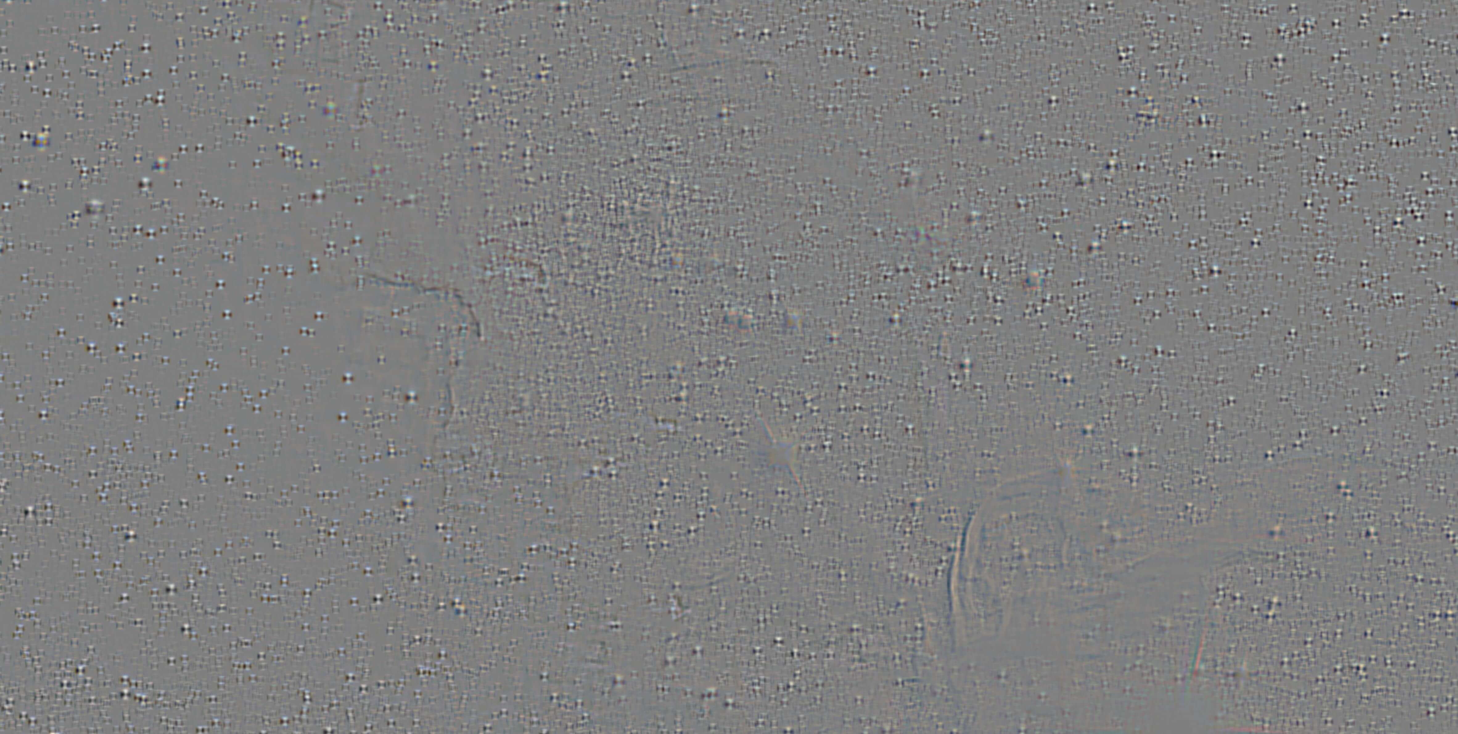
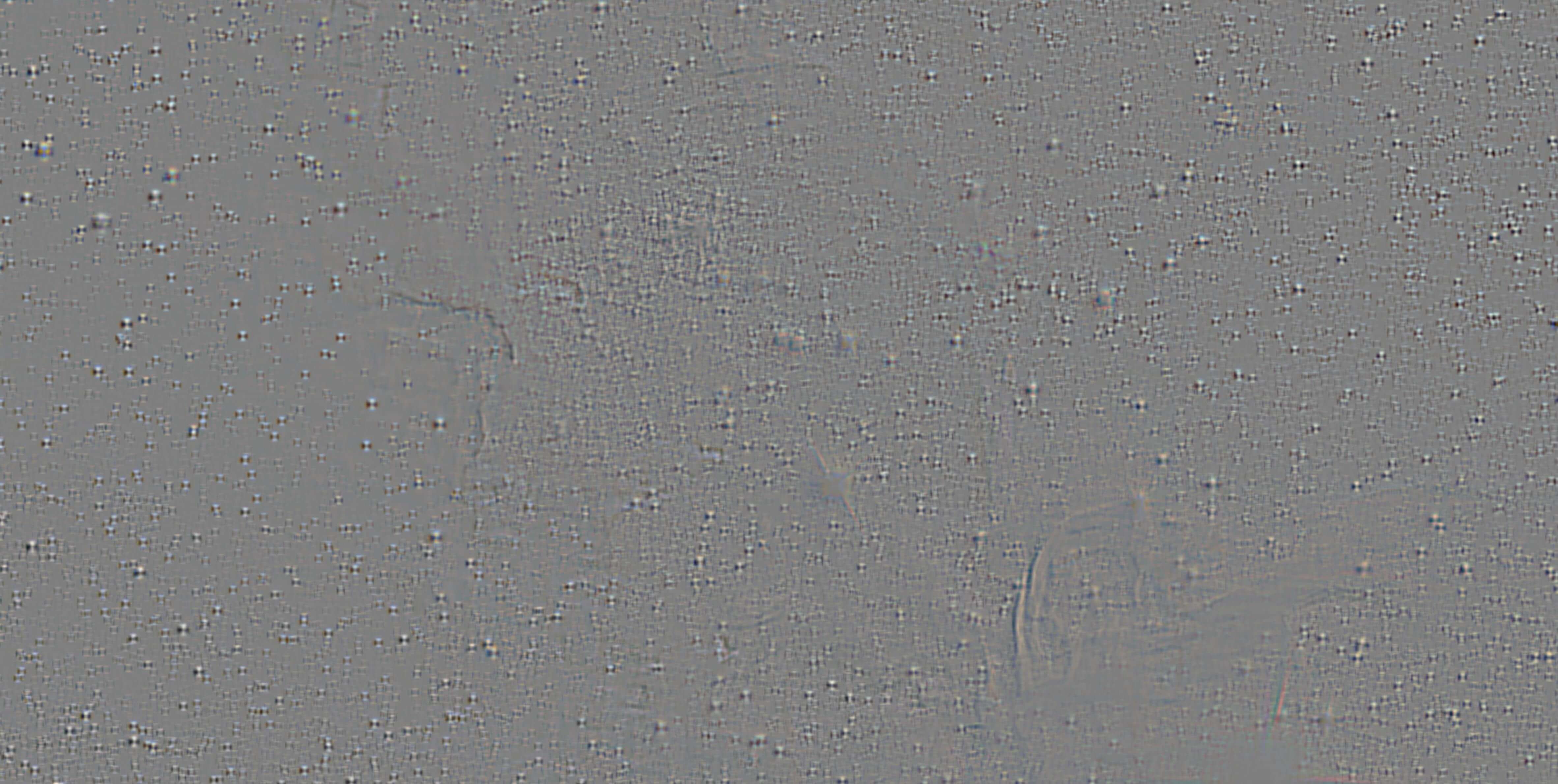
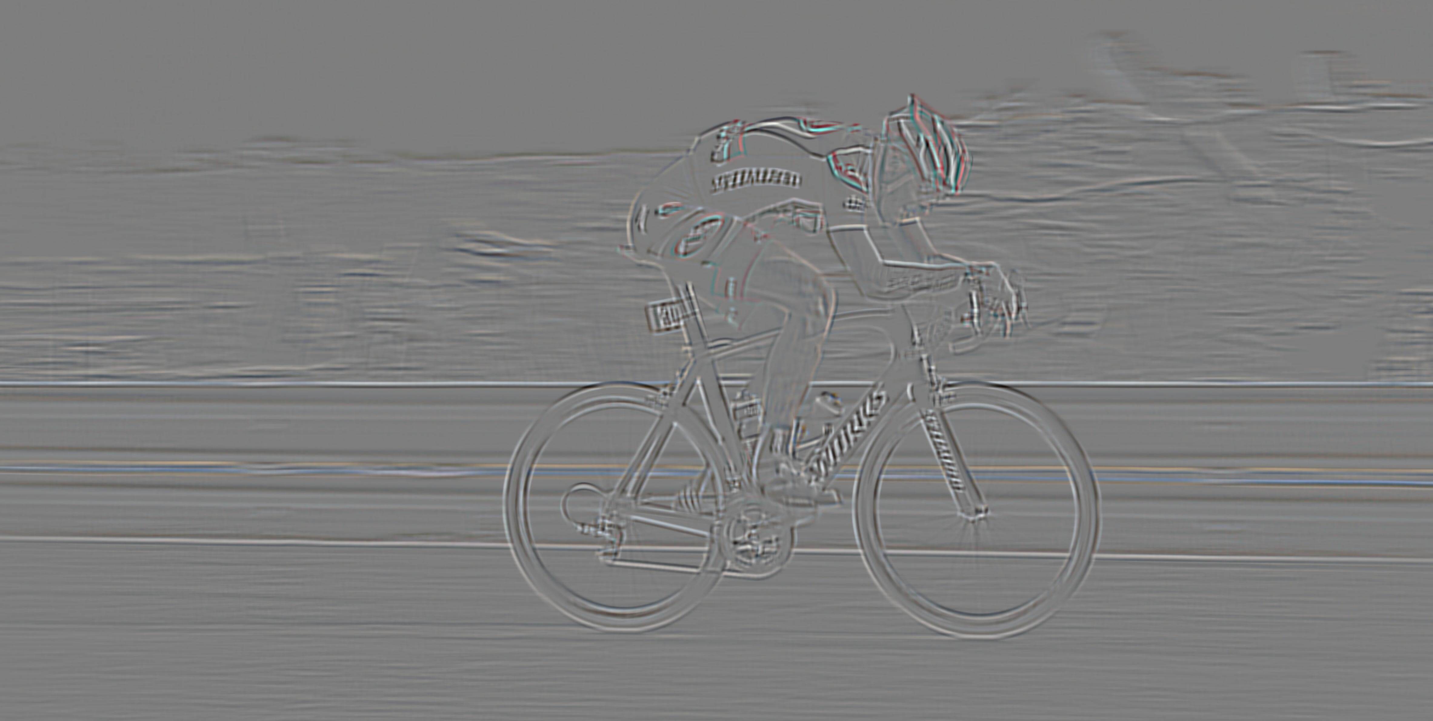
Laplacian stack (space)
|

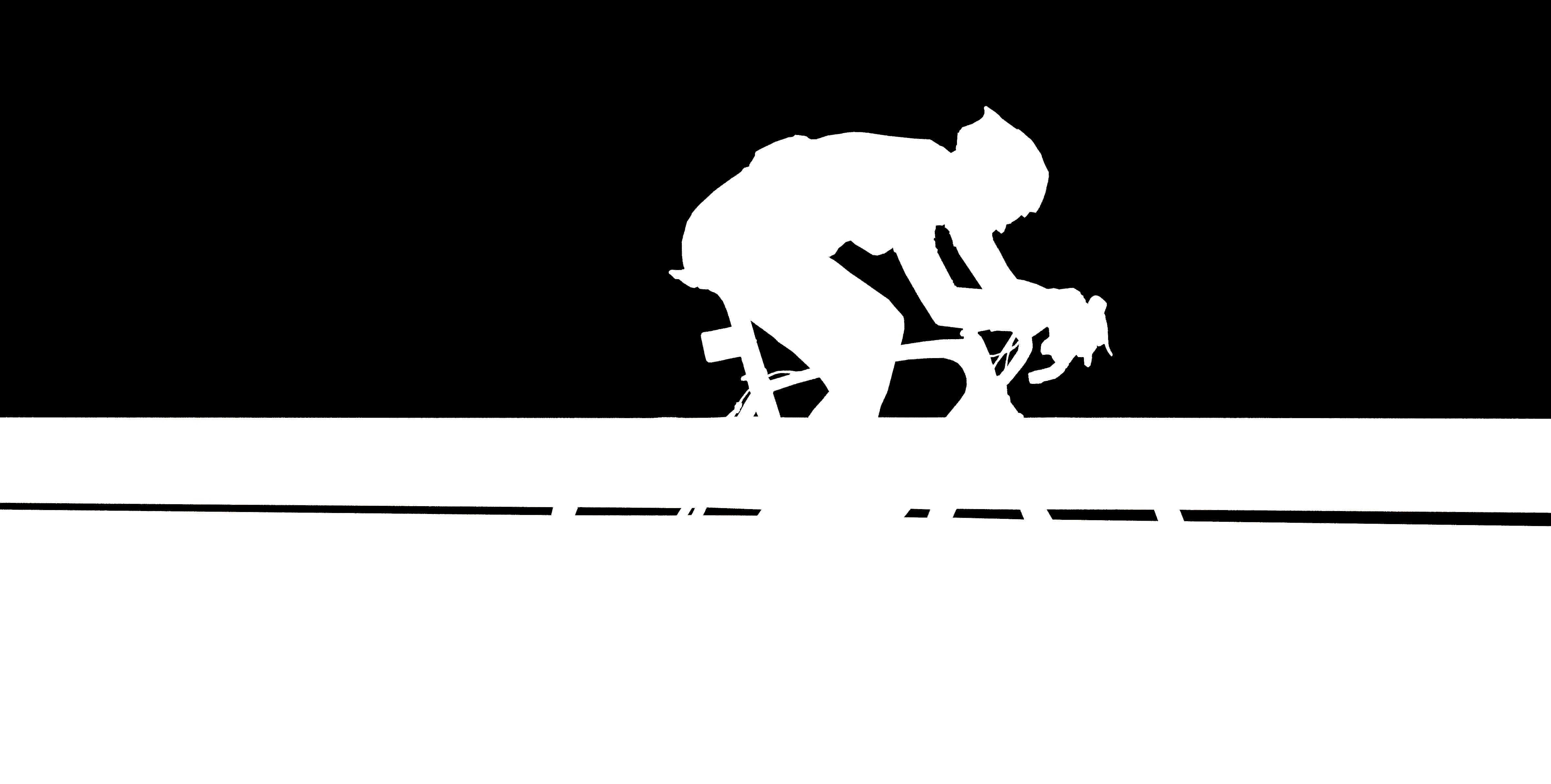
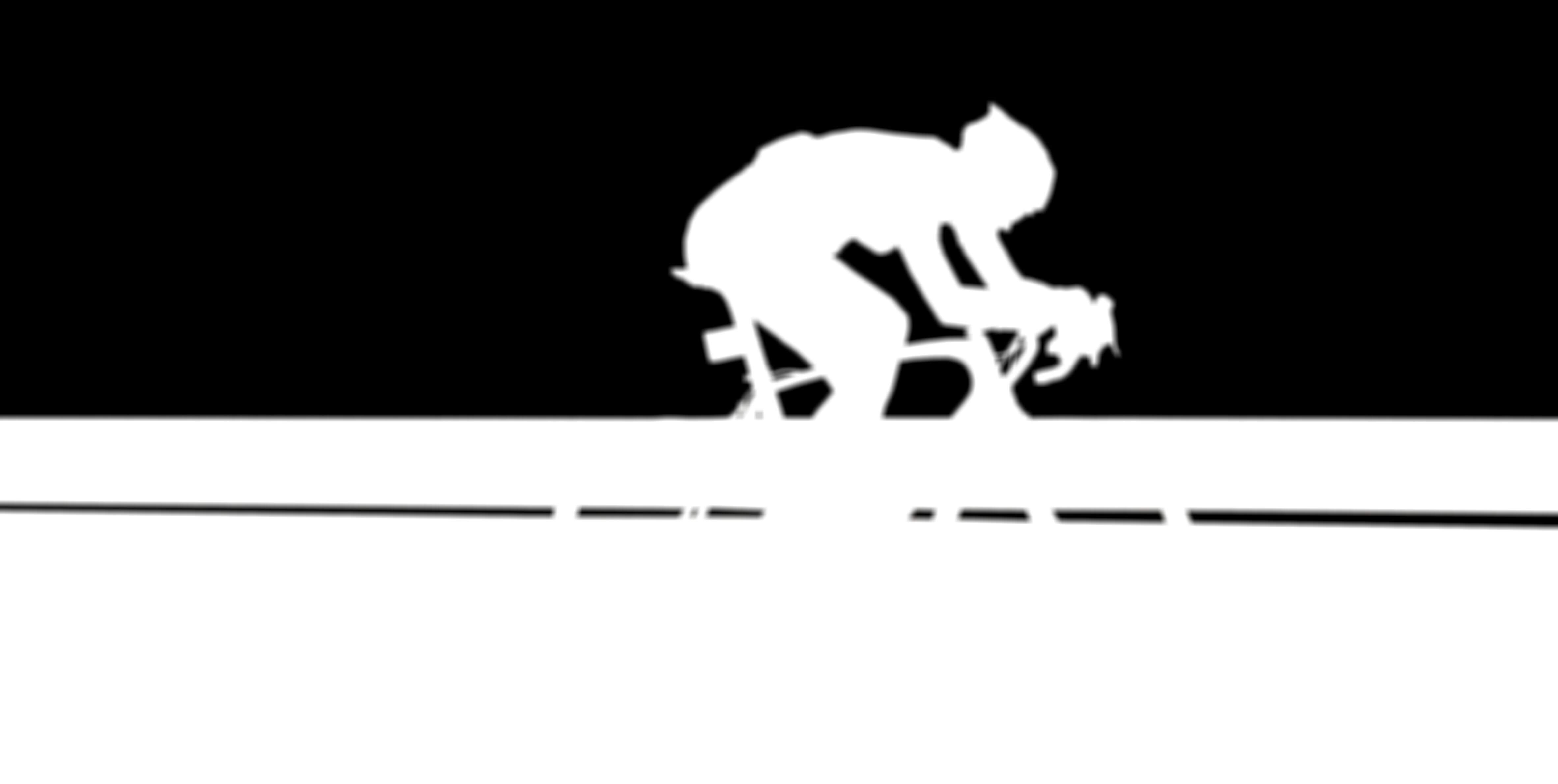
Gaussian stack (mask)
|

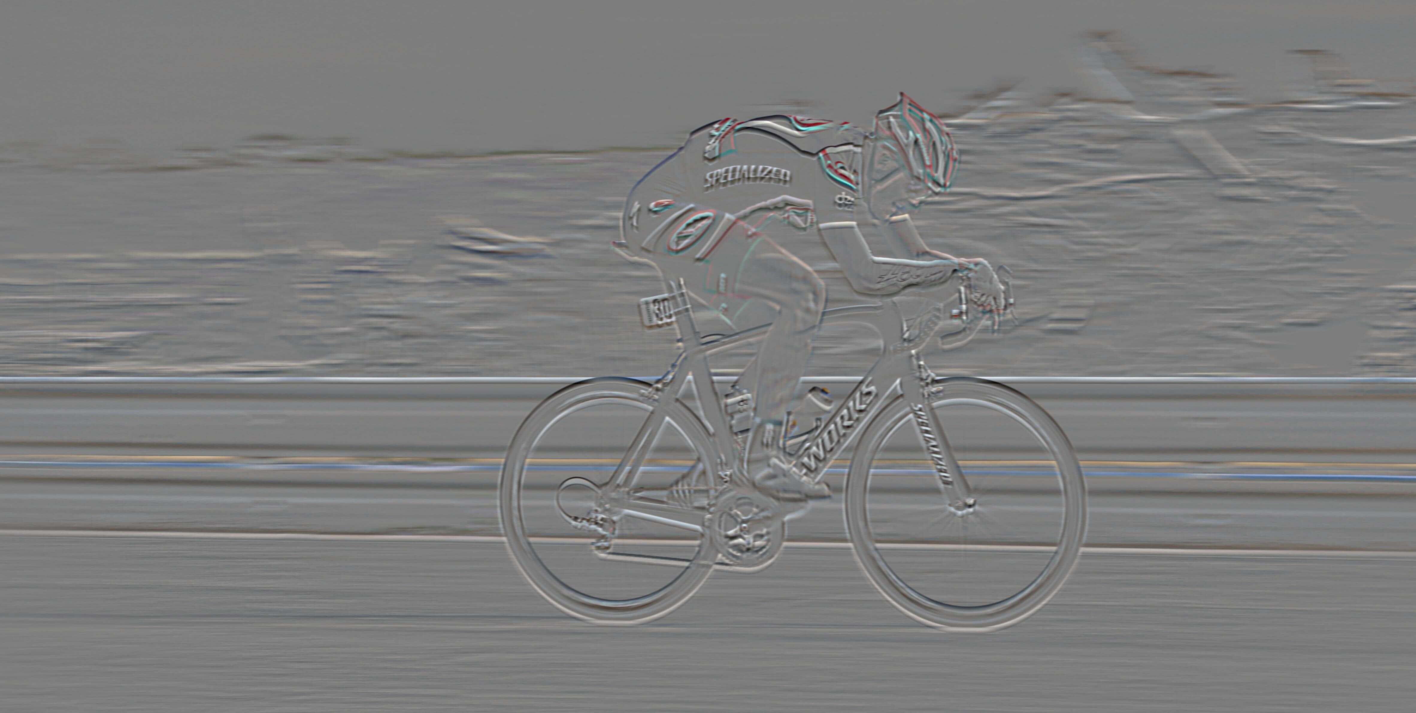
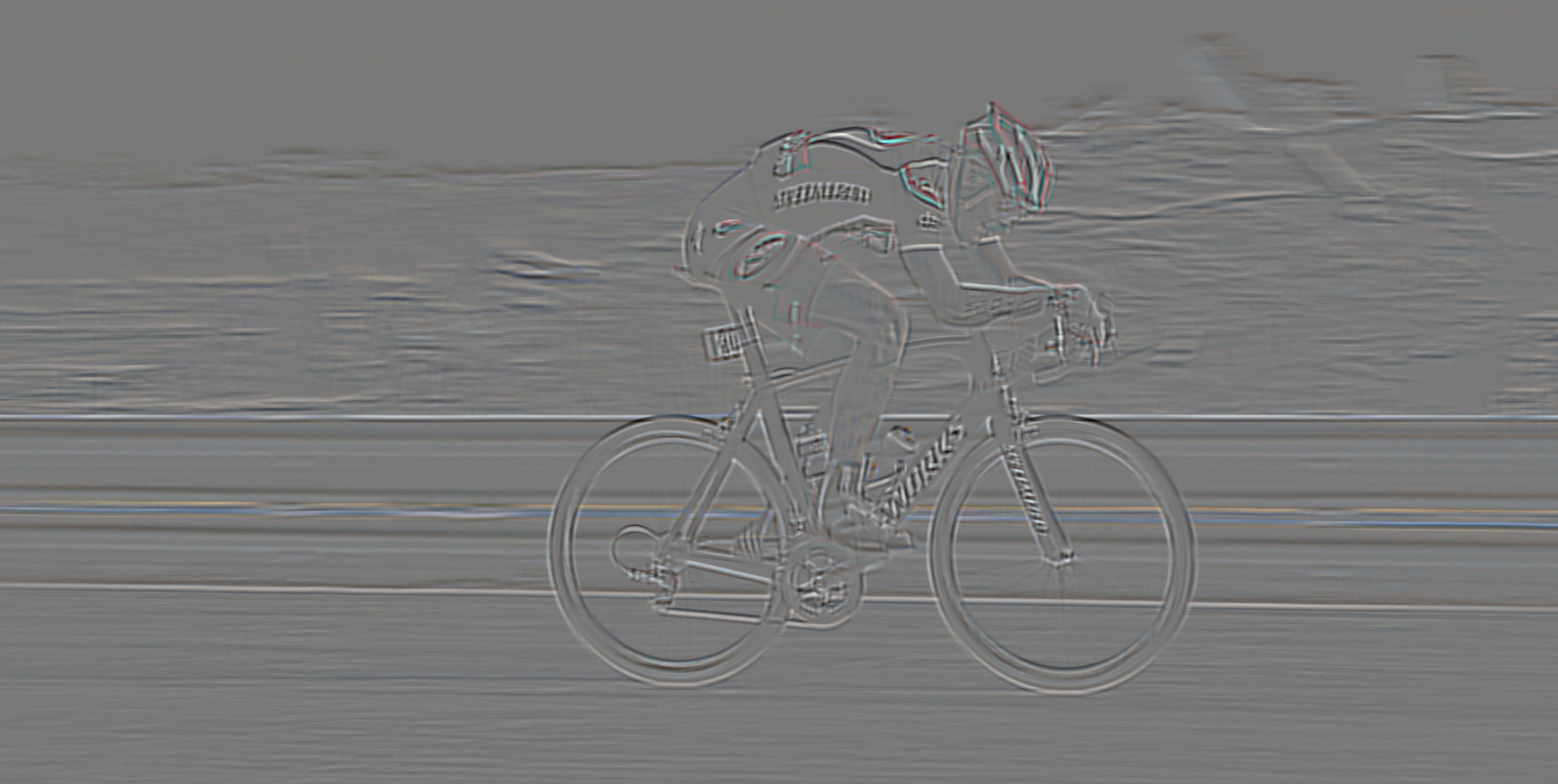
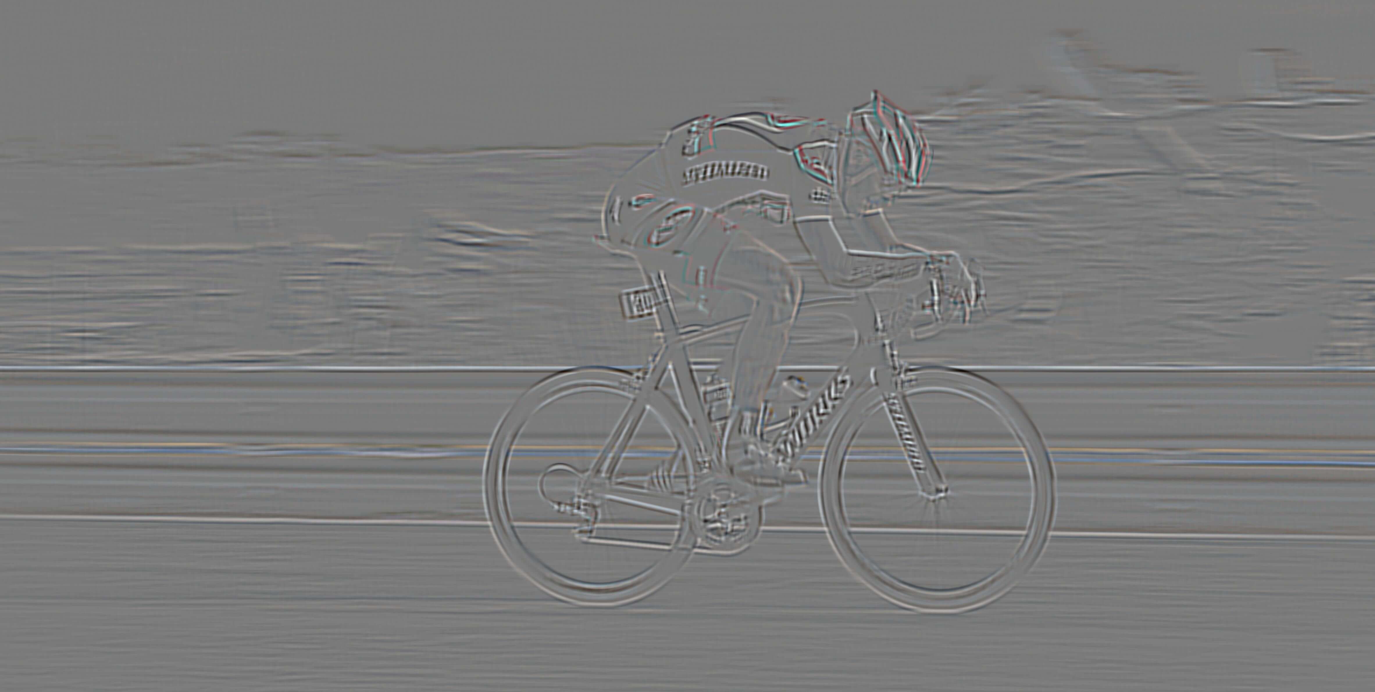
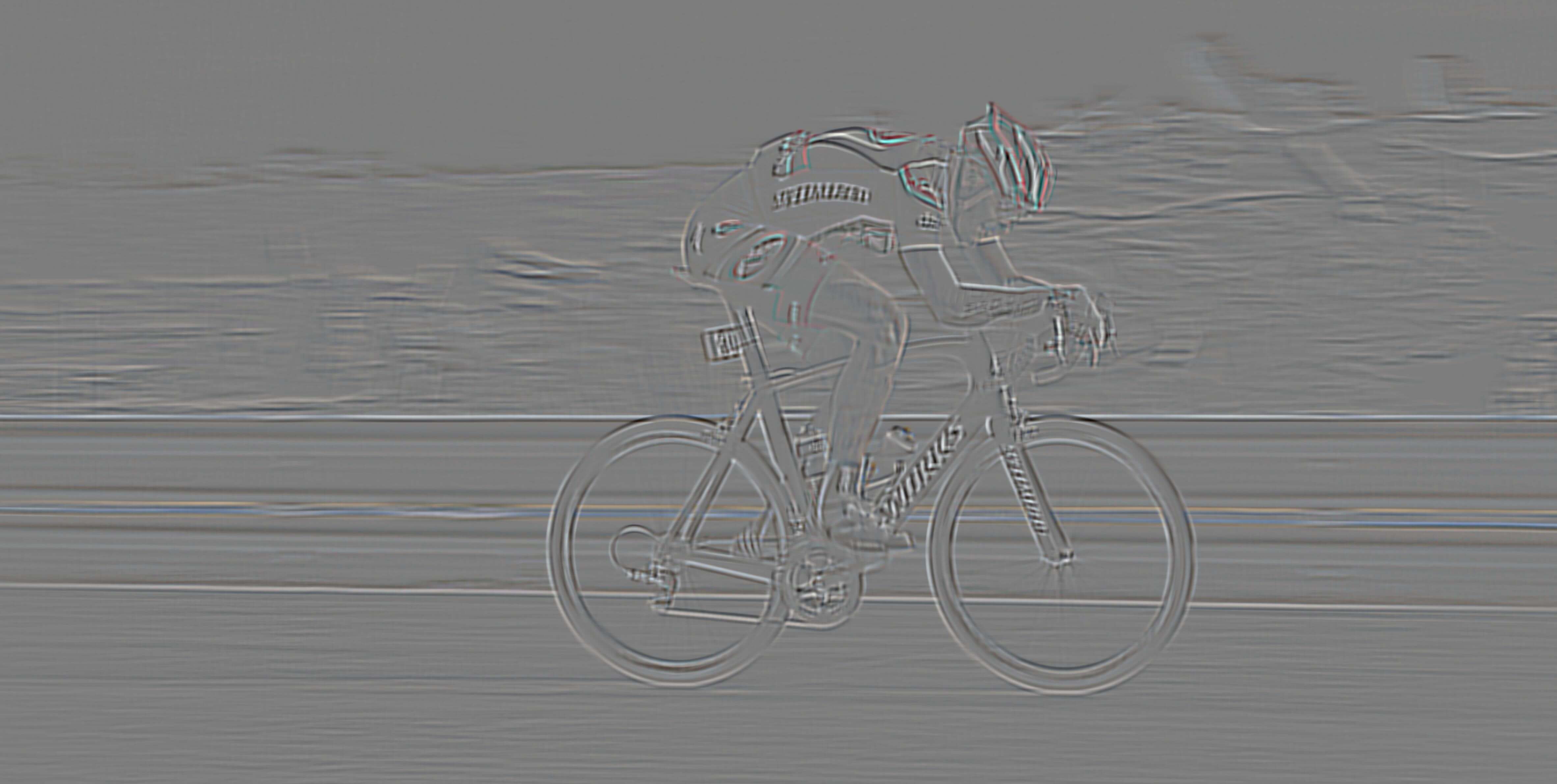
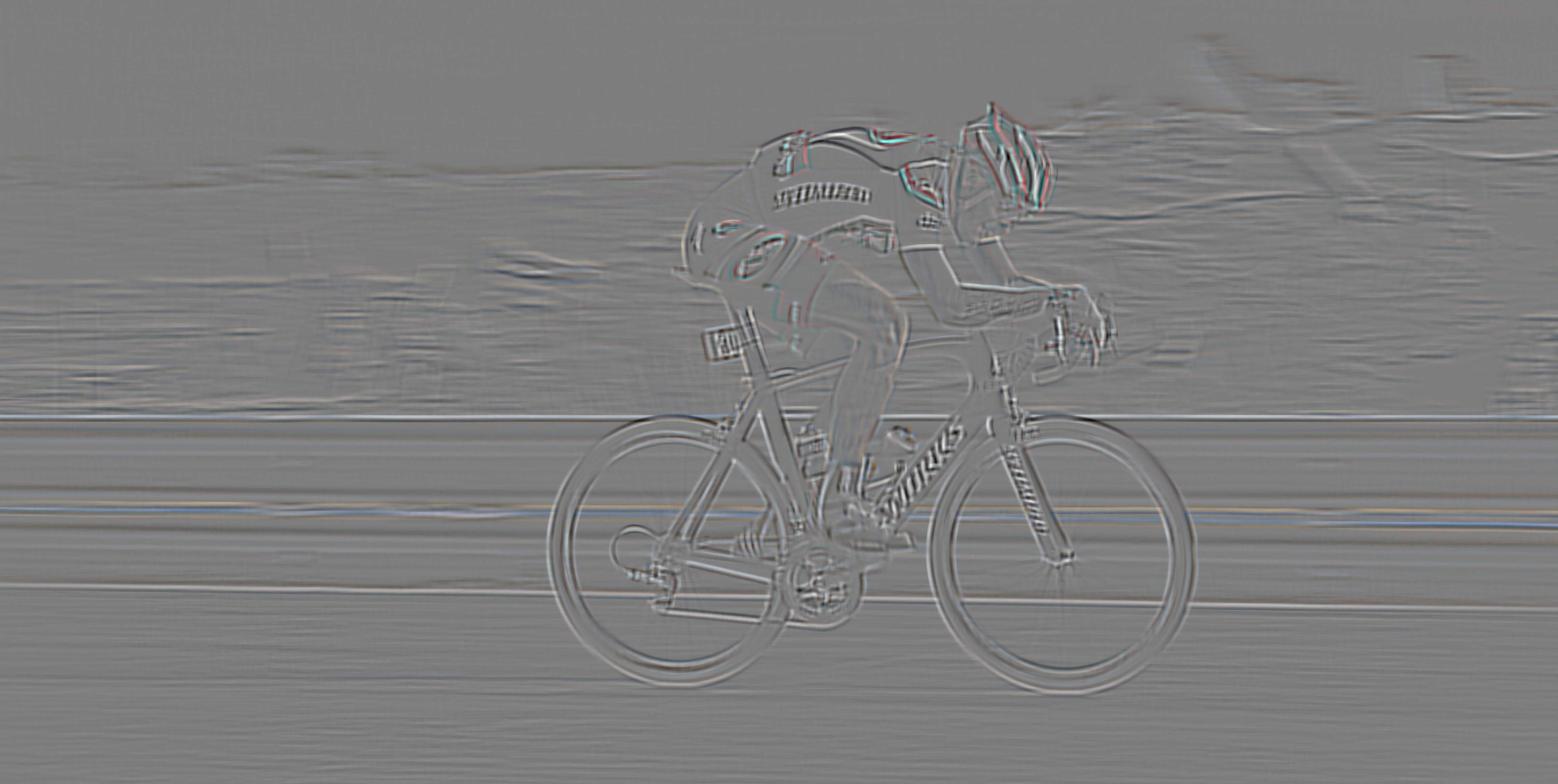
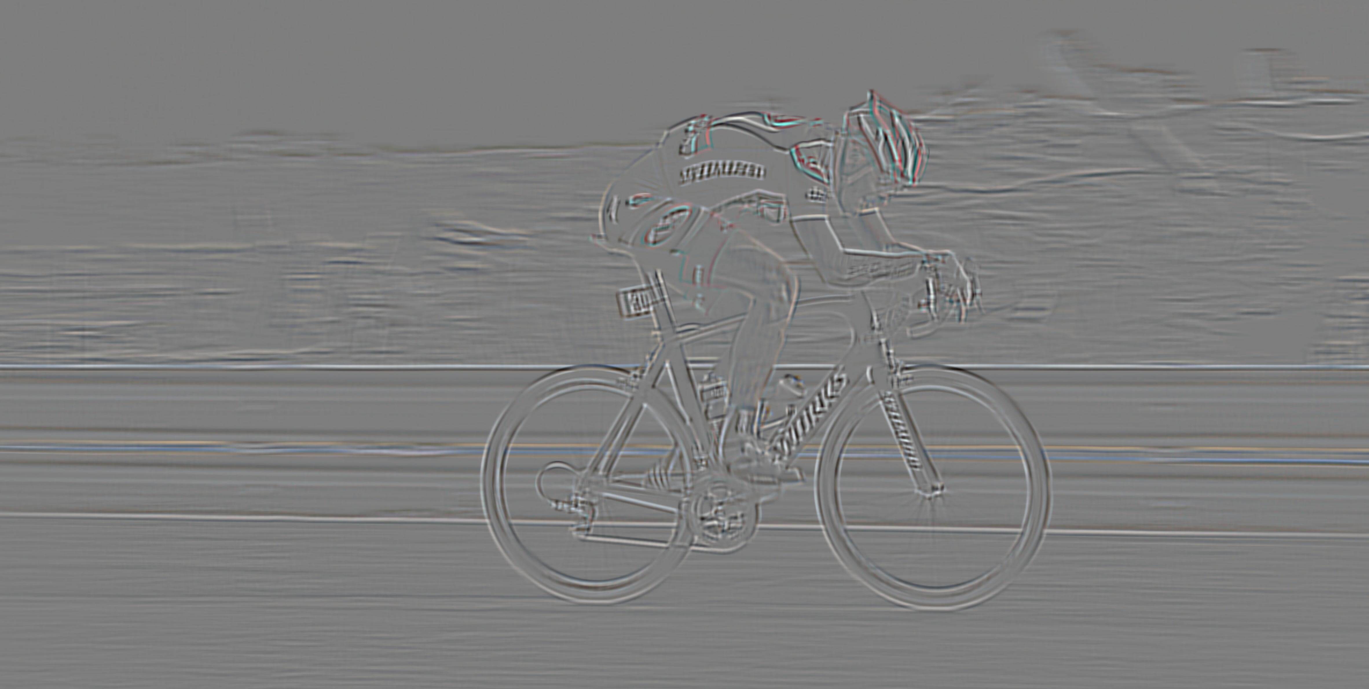
Laplacian stack (biker)
|
This Laplacian image was one of the highlights of the project
|
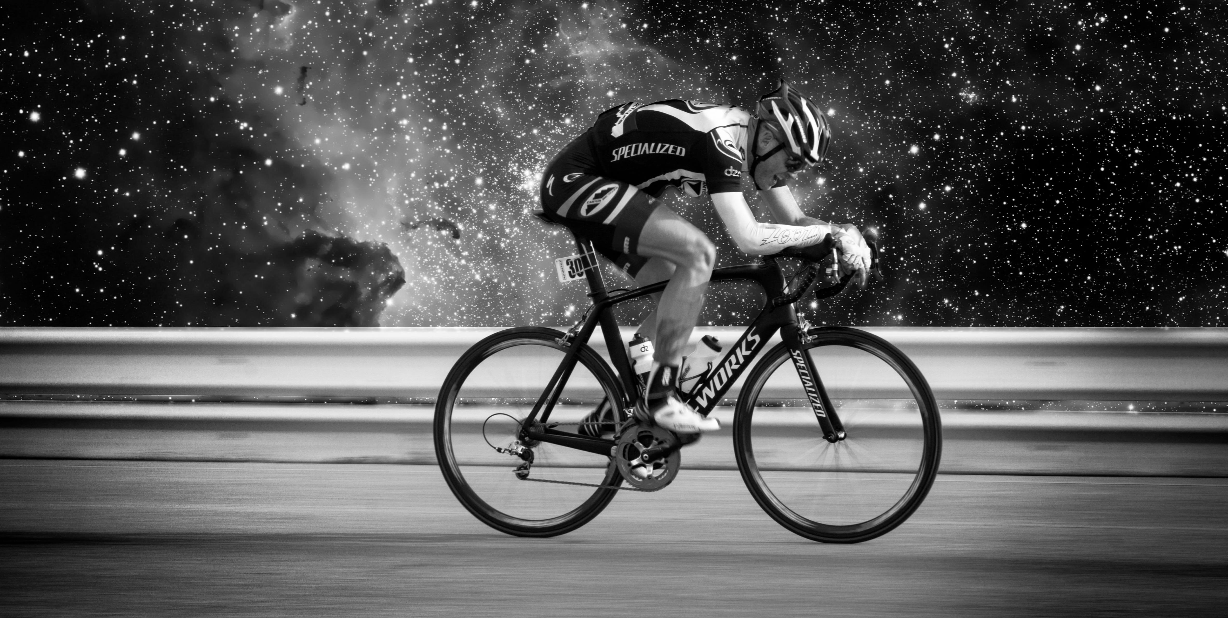
The blended image (biking in space!), grayscale
|
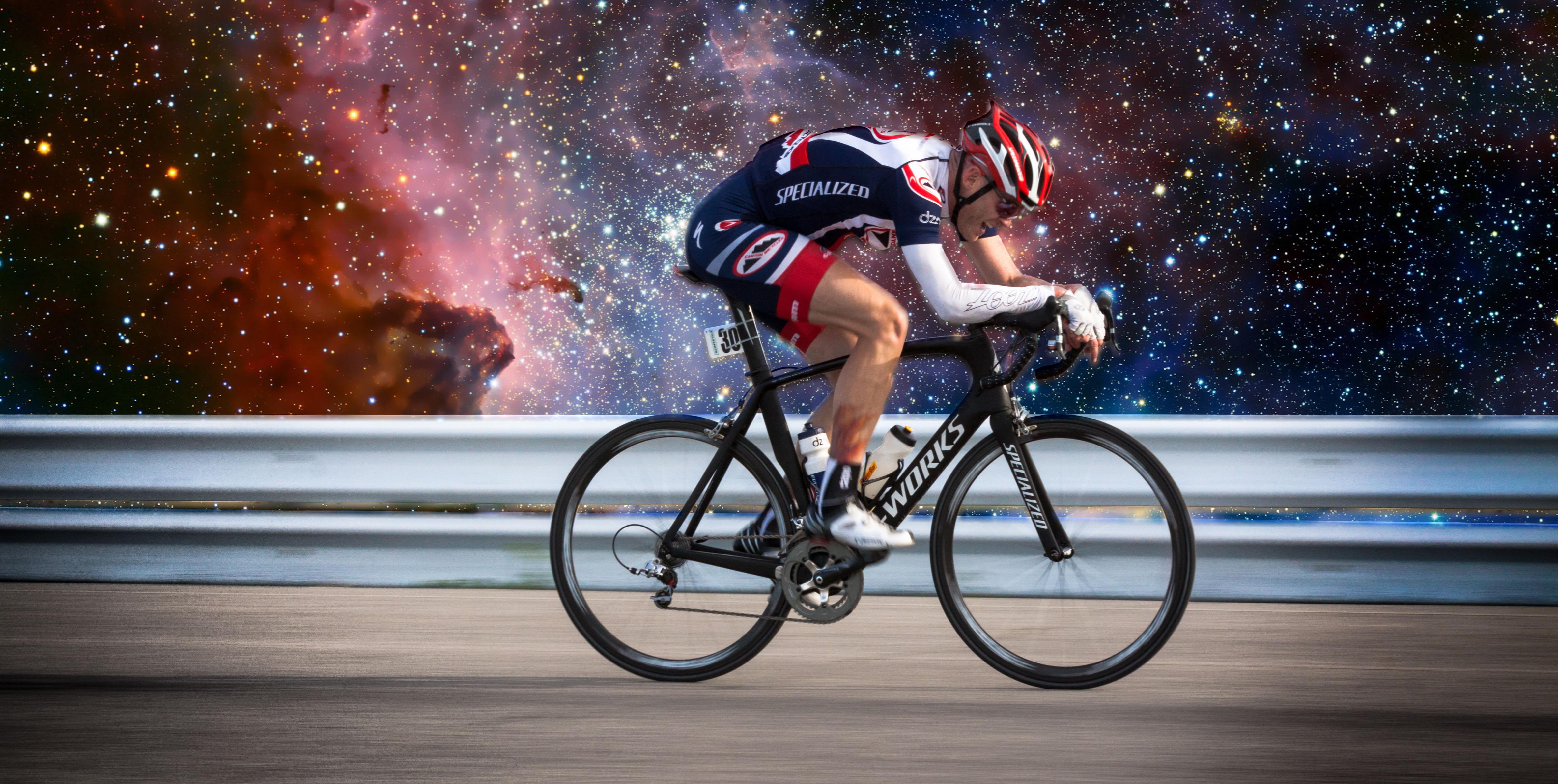
Multiresolution blending... in color!
|
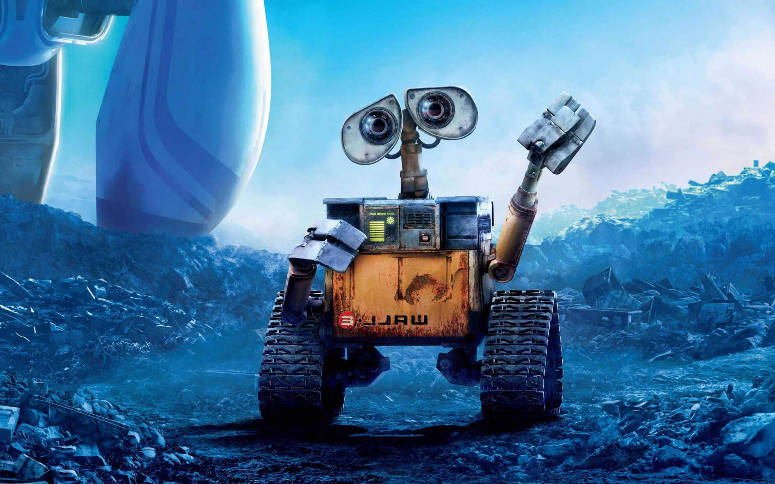
Wall-E
|
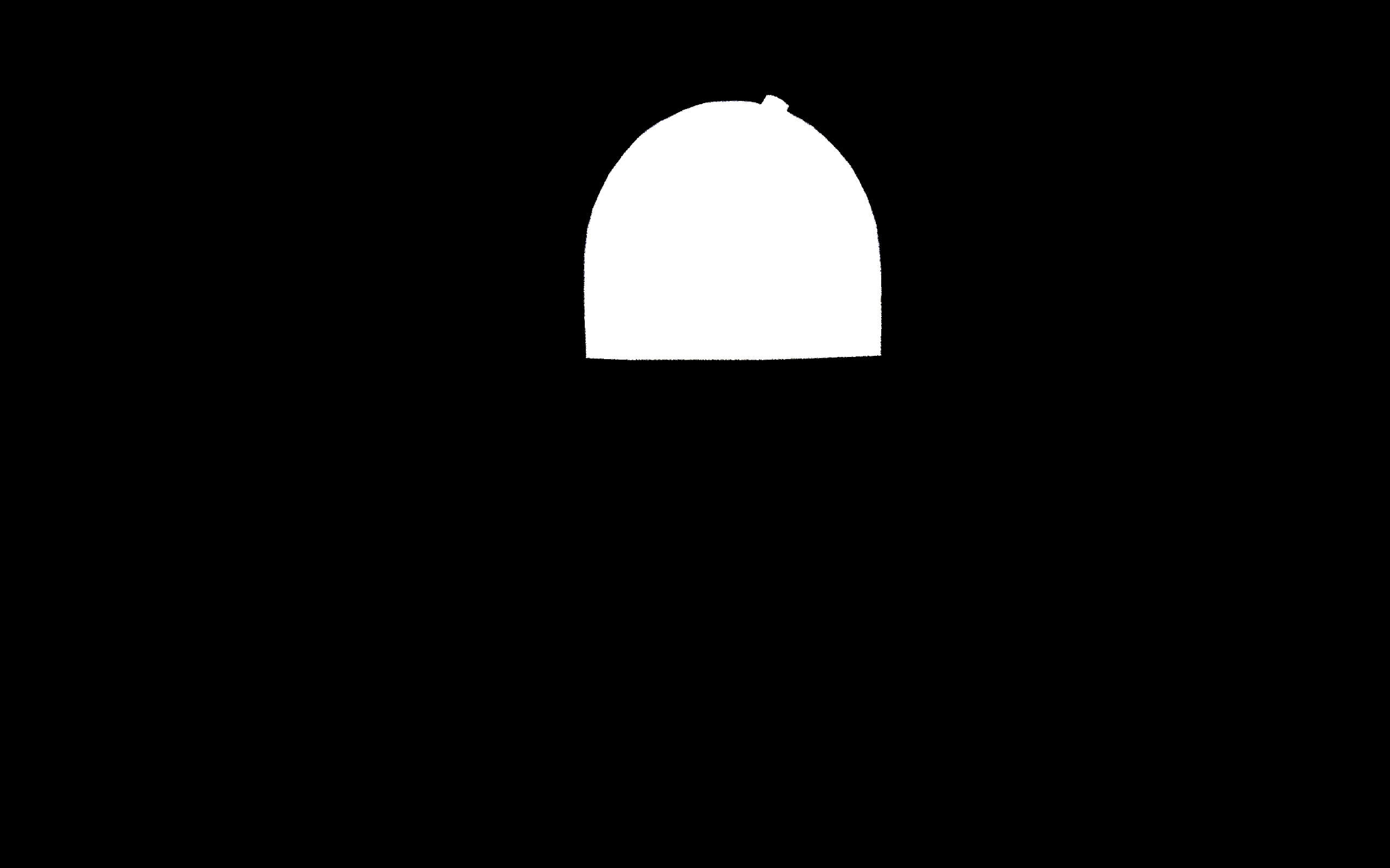
Mask for R2-D2's head
|
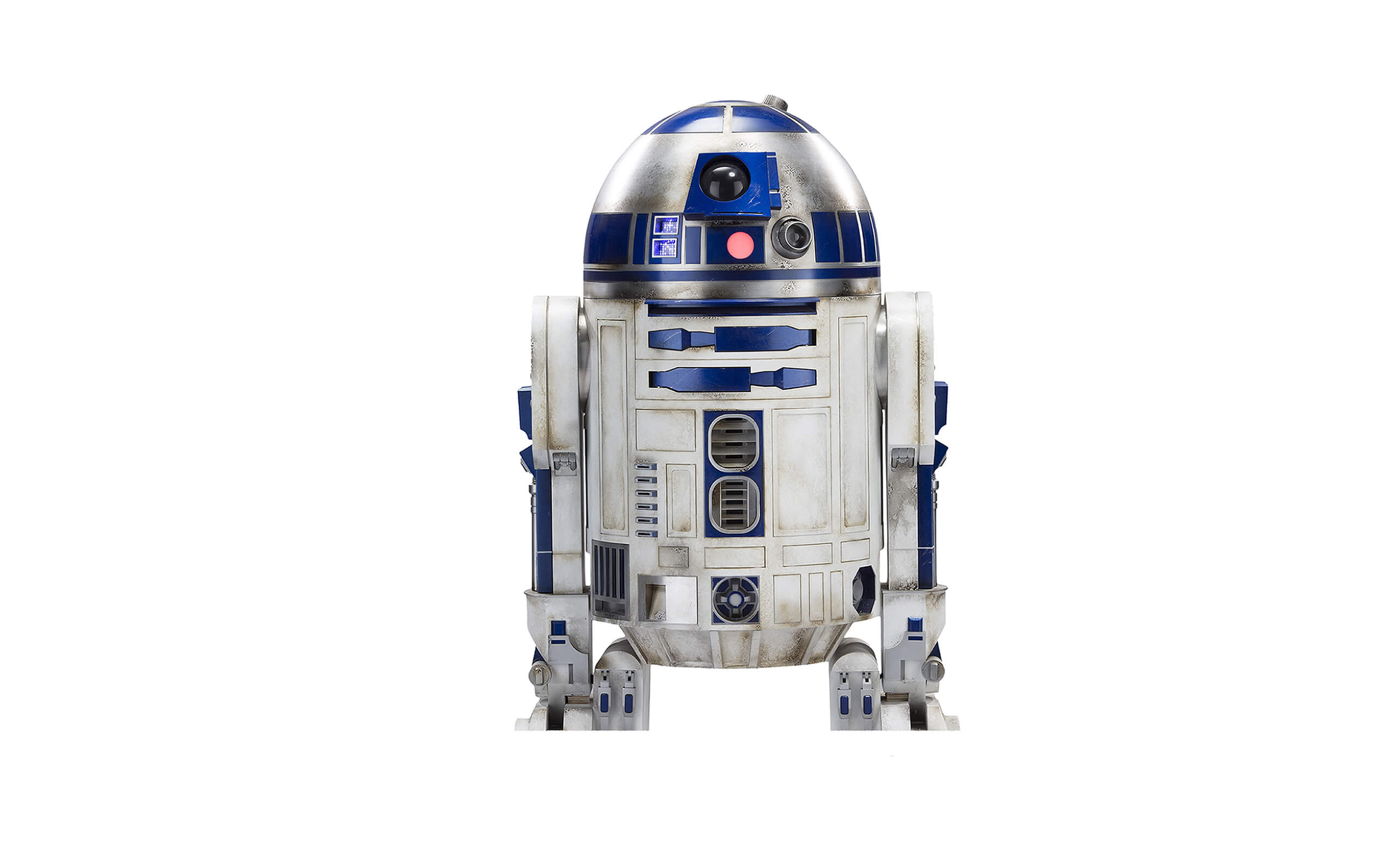
R2-D2
|
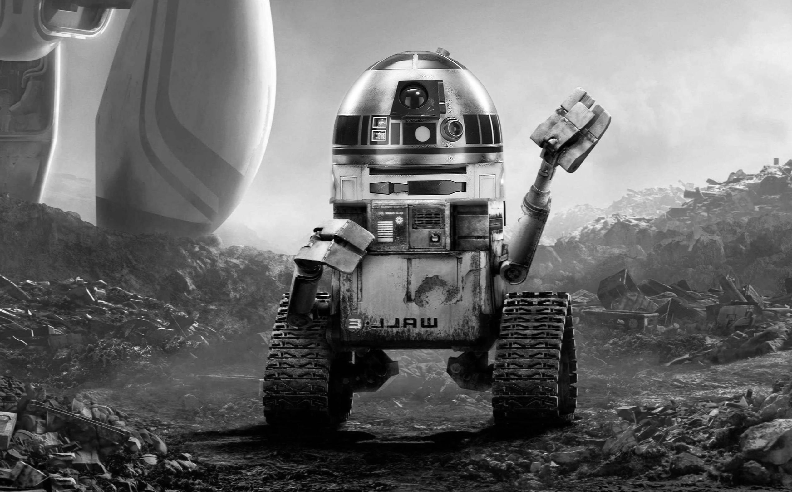
Wall-2D2 (gray)
|
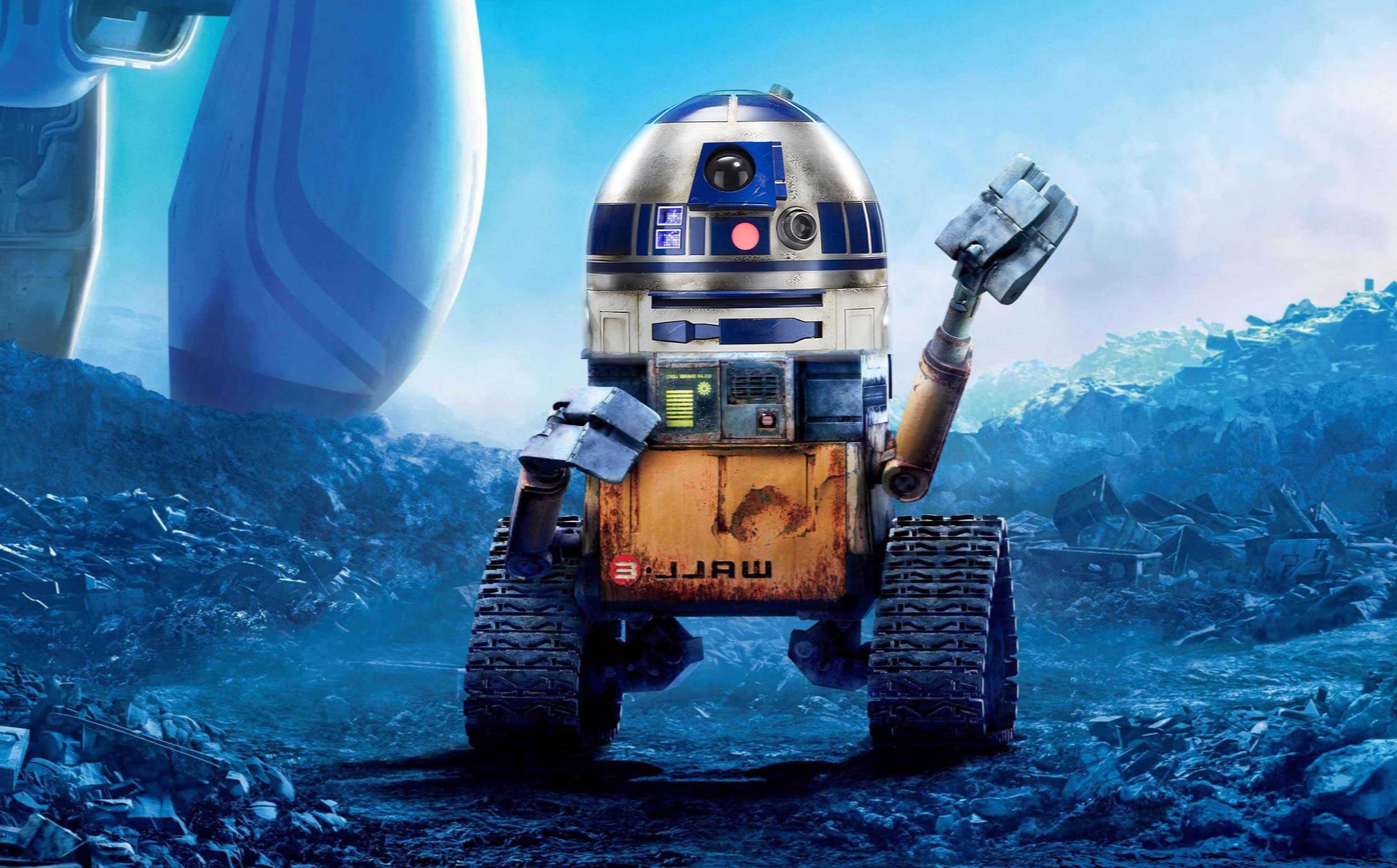
Wall-2D2
|
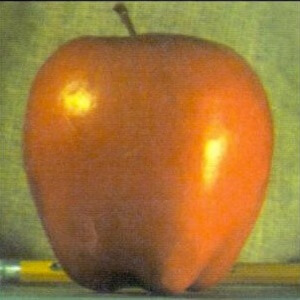
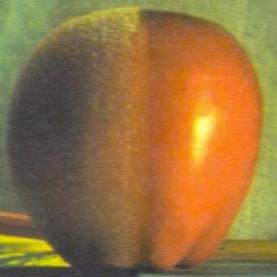
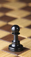
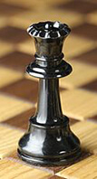
Failure: Mixing the pawn and the queen (below) didn't work very well because the two objects were very different in height and "seamless blending" can only do so much. The top of the queen ended up getting merged with the chessboard instead of the pawn, which did not really have the desired effect.
Bells and Whistles
As shown in pretty much all of the pictures above, multiresolution blending has also been implemented in color. This means that when forming an image in the Gaussian stack (a requirement for building the Laplacian stack, of course!), each of the color channels is convolved with the Gaussian individually, and then all three of the filtered channels are accumulated in order to create a color image for the stack.
Image and Information References [+ Reflection]
Sadly, I have never swum with turtles or (perhaps not as sadly?) met Donald Trump or Hillary Clinton face-to-face. So a huge shout-out to the following sources for the images used in this project! In order of appearance:
I also owe a big thanks to the University of Edinburgh for getting me up to speed on this stuff... after I missed most of the frequency lectures, that is. Praise Edinburgh!
Reflection
And to close this project off, I just want to say that it was incredible to be able to bypass Photoshop and perform sharpening and blending operations through Python code. I always thought of analogous Photoshop effects as being kind of esoteric and magical, but this project has definitely helped me understand how they work beneath the surface. It was pretty mind-blowing (especially for someone without much of a prior background in signal processing) to get a glimpse into that magic, and to see how such simple frequency manipulations can affect images so smoothly and comprehensively! (My favorite part of the assignment, incidentally, was the multiresolution blending. Given more time, I would have liked to try and use the technique to composite multiple images in succession.)